Autoencoder identical to POD
Build a Linear Autoencoder (LAE) comparable to Proper orthogonal decomposition (POD) in two ways. The modes extracted by the two algorithms are compared on the wide (MINST [28*28, 60000]) and slim (Flow past cylinder snapshots [465*354, 110]) datasets. In addition, several regularization methods to improve the orthogonality and optimality of LAE modes are proposed and tested.
Theories
The relation between POD and equivalent linear Autoencoder is first identified by M Milano et.al[1]. They use the nonlinear Autoencoder extension for reconstruction and prediction for near wall turbulence flow. And it has been seen as the first application of neural networks into the field of fluid mechanics[2].
POD/PCA and SVD
A more detailed description can be found in the last post. Only the essence of it is shown below.
Consider a vector space \(\mathbf{X}\in\mathbb{R}^{m\times n}\) as \(\mathbf{X}=\left[\begin{array}{llll}x^1 & x^2 & \ldots & x^n\end{array}\right]\), where \(x^i=\left[\begin{array}{llll}x^i_1 & x^i_2 & \ldots & x^i_m\end{array}\right]^T\). The reduced-order representation \(\tilde{\mathbf{X}}\in \mathbb{R}^{m\times n}\) can be established by POD as: \[ \tilde{\mathbf{X}}=\sum_{i=1}^p \alpha_i \boldsymbol{\phi}_i=\boldsymbol{\Phi} \boldsymbol{\alpha},\qquad \tilde{\mathbf{X}}\in\mathbb{R}^{m\times n}, \mathbf{\Phi}\in\mathbb{R}^{m\times p}, \boldsymbol{\alpha}\in\mathbb{R}^{p\times n} \] where the columns of \(\mathbf{\Phi}\) is called modes representing the optimal set of basis spanned by which the reconstructed space \(\tilde{\mathbf{X}}\) has mathematically the lowest \(L2\) loss to the original space \(\mathbf{X}\).
These modes can be extracted by SVD (or efficient SVD): \[ \mathbf{X} = \mathbf{U}\boldsymbol{\Sigma}\mathbf{V^T},\qquad \mathbf{U}\in\mathbb{R}^{m\times m}, \boldsymbol{\Sigma}\in\mathbb{R}^{m\times n}, \mathbf{V}\in\mathbb{R}^{n\times n} \] And the reduced order representation can be reconstructed as: \[ \tilde{\mathbf{X}} = \underbrace{\tilde{\mathbf{U}}}_{\boldsymbol{\Phi}}\underbrace{\tilde{\boldsymbol{\Sigma}}\tilde{\mathbf{V}}^\mathbf{T}}_{\boldsymbol{\alpha}},\qquad \tilde{\mathbf{U}}\in\mathbb{R}^{m\times p}, \tilde{\boldsymbol{\Sigma}}\in\mathbb{R}^{p\times p}, \tilde{\mathbf{V}}\in\mathbb{R}^{n\times p} \] where \(\tilde{\mathbf{U}}, \tilde{\mathbf{V}}\) is the first \(p\) columns of \(\mathbf{U},\mathbf{V}\) respectively. \(\tilde{\boldsymbol{\Sigma}}\) is the first \(p\) dimensional diagonal sub-matrix of \(\boldsymbol{\Sigma}\). Relating to POD, we have \(\boldsymbol{\Phi} = \tilde{\mathbf{U}}\) and \(\boldsymbol{\alpha} = \tilde{\boldsymbol{\Sigma}}\tilde{\mathbf{V}}^\mathbf{T}\).
Linear autoencoder (LAE)
One-layer linear neural network (without nonlinear activation function layer) can be concluded with an input data \(\mathbf{X_0}\in\mathbb{R}^{m\times n}\) and the output \(\mathbf{X_1}\in \mathbb{R}^{p\times n}\): \[
\mathbf{X_1}=\boldsymbol{W_1}\mathbf{X_0} + \mathbf{b_1},\qquad \mathbf{X_1}\in \mathbb{R}^{p\times n}, \mathbf{W_1}\in\mathbb{R}^{p\times m}, \mathbf{X_0}\in\mathbb{R}^{m\times n}, \mathbf{b_1}\in\mathbb{R}^{p\times 1}\text{(broundcast)}
\] 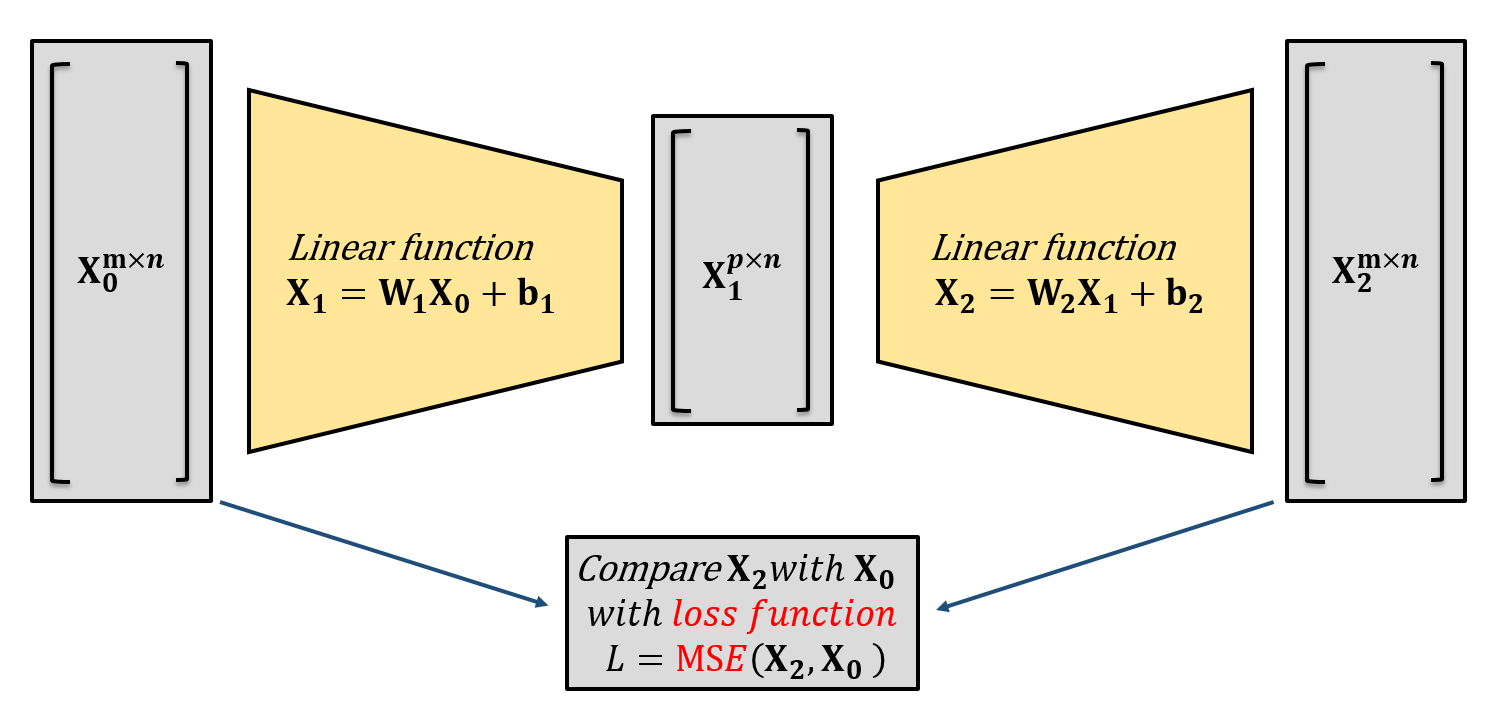
As the architecture shown above, a linear autoencoder stacks two of linear layer with a lower dimensional intermediate output acting as a bottleneck, also called the latent space. The first and second layer of the autoencoder are always referred to as the encoder and decoder.
With a well trained LAE, the original input data \(\mathbf{X_0}\) can be reconstructed from a latent space \(\mathbf{X_1}\), the error between original data \(\mathbf{X_0}\) and the reconstructed data \(\mathbf{X_2}\) can be minimized regressively via back propagation and gradient descent. When choosing mean square error (MSE) as error/loss function, the optimal latent space extracted by the optimal LAE is identical with that extracted by POD/PCA.
Equivalent LAE to POD
Straightforward method
To get a autoencoder equivalent to POD, set \(\mathbf{b_1} = \mathbf{b_2}=0\), a straightforward way is to make the auto encoder process \(\mathbf{X}\) and reconstruct it as \(\tilde{\mathbf{X}}\). The mathematical representation is: \[ \begin{aligned} layer1: \qquad \mathbf{X_1}=\boldsymbol{W_1}{\color{purple}\mathbf{X}},&\qquad \mathbf{X_1}\in \mathbb{R}^{p\times n}, \mathbf{W_1}\in\mathbb{R}^{p\times m}, \mathbf{X}\in\mathbb{R}^{m\times n} \\ layer2: \qquad {\color{purple}\tilde{\mathbf{X}}}=\boldsymbol{W_2}\mathbf{X_1},&\qquad \tilde{\mathbf{X}}\in \mathbb{R}^{m\times n}, \mathbf{W_2}\in\mathbb{R}^{m\times p} \end{aligned} \] associated with the above symbols, the weights of the second layer are used as the modes i.e. \[ \begin{aligned} \boldsymbol{\Phi} &= \mathbf{W_2} \\ \boldsymbol{\alpha} &= \mathbf{X_1} \end{aligned} \]
Transposition method
Although, there is another equivalence, if we make the autoencoder process a transposition of data, we have a bottleneck mapping from \(\mathbf{X'}\) to \(\tilde{\mathbf{X}}'\): \[ \begin{aligned} layer1: \qquad \mathbf{X_1'}=\boldsymbol{W_1}'{\color{purple}\mathbf{X}'},&\qquad \mathbf{X_1'}\in \mathbb{R}^{p\times m}, \mathbf{W_1'}\in\mathbb{R}^{p\times n}, \mathbf{X'}\in\mathbb{R}^{n\times m} \\ layer2: \qquad {\color{purple}\tilde{\mathbf{X}}'}=\boldsymbol{W_2}'\mathbf{X_1'},&\qquad \tilde{\mathbf{X}}\in \mathbb{R}^{n\times m}, \mathbf{W_2'}\in\mathbb{R}^{n\times p} \end{aligned} \] In this case, we have the intermediate latent space related to the modes, that is \[ \begin{aligned} \boldsymbol{\Phi} &= \mathbf{X_1'} \\ \boldsymbol{\alpha}&= \mathbf{W_2'} \end{aligned} \]
Improvement
Well, those equivalences only exist in imagination because of the large freedom of gradient descend process
- non-orthogonality: modes extracted by LAE is not necessarily orthogonal
- non-optimality: (L2) energy preserved by the modes are not ranked in descending order
There might be several methods to obtain a set of modes comparable with the POD modes:
- Two-stage:
[method 1]run another SVD on the raw modes extracted by the LAE, it works on both the two methods.
- End-to-end:
- Straightforward method
[method 2]Orthonormal regularization on the weight[method 3]Orthogonalized the weight every step (parameterization)[method 4]SVD the weight every step (custom SVD parameterization)
- Transpose method
[method 5]Add an SVD layer after the 1st layer output.
- Straightforward method
All these improvements will be compared and tested in the case study section. In this section, the [method 2] regularization methods and the [method 4] SVD parameterization will be further talked about.
L2 regularization
Before introducing the orthogonal regularization used in [method 2], let's recall the popular L2 regularization. For dataset \(\mathbf{X}\in\mathbb{R}^{m\times n}\) as \(\mathbf{X}=\left[\begin{array}{llll}x^1 & x^2 & \ldots & x^n\end{array}\right]\), where \(x^i=\left[\begin{array}{llll}x^i_1 & x^i_2 & \ldots & x^i_m\end{array}\right]^T\), the L2 regularized loss function of the 2-layer linear autoencoder is: \[
\begin{aligned}
\mathbf{\hat{\mathcal{L}}_{(W_1,W_2)}} &= \mathcal{L}_{ms} + \mathcal{L}_{L2} \\
\text{where:}\qquad {\mathcal{L}_{ms}}_{\mathbf{(W_1,W_2)}} &= \frac{1}{n}\sum_{i=1}^{n} MSE(\mathbf{\tilde{x^{i}},x^{i}}), \\
{\mathcal{L}_{L2}}_{\mathbf{(W_1,W_2)}} &=\frac{\lambda_{L2}}{2n}\sum_{l=1}^2 (\left\|\mathbf{W}_{l}\right\|^2_F), \\
\left\|\mathbf{W}_1\right\|^2_F &=\sum_{i=1}^{p}\sum_{j=1}^{m}{\mathbf{W}_1}_{i}^{j2} = trace(\mathbf{W}^T_1\mathbf{W}_1), \\
\quad \left\|\mathbf{W}_2\right\|^2_F &= \sum_{i=1}^{p}\sum_{j=1}^{m}{\mathbf{W}_2}_i^{j2} = trace(\mathbf{W}^T_2\mathbf{W}_2)
\end{aligned}
\]
Normally, the L2 regularization is not applied by tailoring the loss function, but more simply and efficiently, the weight updating process, referring as the weight decay.
In the gradient descend algorithm, weights are updated by the gradient of loss function w.r.t. the weights: \[\mathbf{W}_l = \mathbf{W}_l-\alpha \frac{\partial{\hat{\mathcal{L}}}}{\partial\mathbf{W}_l}\] With \(\hat{\mathcal{L}} = \mathcal{L}_{ms} + \mathcal{L}_{L2}\), we have: \[\begin{aligned}\mathbf{W}_l &= \mathbf{W}_l-\alpha \left(\frac{\partial\mathcal{L}_{ms}}{\partial\mathbf{W}_l}+\frac{\partial\mathcal{L}_{L2}}{\partial\mathbf{W}_l}\right) \\&= \mathbf{W}_l-\alpha \left(\frac{\partial\mathcal{L}_{ms}}{\partial\mathbf{W}_l}+\frac{\lambda_{L2}}{n}\mathbf{W}_l\right) \\\end{aligned}\] And \(\lambda_{L2}\) is called the weight decay parameter, with \(\alpha\) being the learning rate.
We can't do such simplification with other regularization methods.
Ablation tests on the L2 regularization (weight decay) and learning rate are carried out with MNIST dataset. [method 1] is used to inspect the results. Some interesting results are shown in the Appendix. It turns out that a small L2 regularization leads to more orthogonal modes and lower reconstruction error. Too much L2 regularization leads to high bias/under fitting.
Orthonormal regularization
One attractive property of the POD modes is the (semi) orthonormality, i.e. the modes are independent with each others i.e. the inner product of the mode matrix is identity. \[ \begin{aligned} \boldsymbol{\Phi}^T\boldsymbol{\Phi}&=\mathbf{I}, \qquad\mathbf{I} \text{ is the identity matrix} \\ \left\langle \phi_i, \phi_j\right\rangle &= \delta_{i j}, \qquad\forall i, j \end{aligned} \] To impose an orthonormal penalty on the weight of LAE, mimicking the L2 regularization, we can design an orthonormal regularization: \[ {\mathcal{L}_{ortho}}_{\mathbf{(W_1,W_2)}} =\lambda_{ortho}\sum_{l=1}^2\left\|\mathbf{W}^T_l\mathbf{W}_l-\mathbf{I}\right\|^2_F \]
Orthogonal regularization is a technique first proposed in CNNs.
Brock et.al first proposed that maintaining an orthogonal weight is desirable when training neural networks. And they proposed the orthogonal regularization in L1 norm [4]. Then they upgraded it to a new variation in BigGAN[5] based on the L2 norm. Lubana et.al[6] applied the same method to the field of neural network pruning[7].
SVD parameterization
Parameterization is a method transforming the parameter of neural network in an appropriate way before using it. For example, orthogonal parameterization orthogonalizes the weight matrix of a layer of the neural network.
Orthogonal parameterization guarantees a arbitrary orthogonal basis, but we want more. So here it is possible to define a SVD parameterization regulating the the decoder such that: \[ \begin{aligned} layer2:& \qquad \tilde{\mathbf{X}}=\boldsymbol{W_2}\mathbf{X_1}= \mathbf{U}\boldsymbol{\Sigma}\mathbf{V^T}\mathbf{X_1} = \boldsymbol{\hat{W_2}}\mathbf{\hat{X_1}} \\ \text{where:}& \qquad \boldsymbol{\hat{W_2}} = \mathbf{U}, \quad \mathbf{\hat{X_1}}=\boldsymbol{\Sigma}\mathbf{V^T}\mathbf{X_1} \\ &\qquad \mathbf{U},\boldsymbol{\Sigma},\mathbf{V} = SVD(\boldsymbol{W_2}) \end{aligned} \] In this case the modes \(\hat{W_2}\) automatically gets singular value decomposed.
Parameterization only affects the weight, i.e. \(\boldsymbol{\hat{W_2}} = \mathbf{U}\) not \(\mathbf{\hat{X_1}}=\boldsymbol{\Sigma}\mathbf{V^T}\mathbf{X_1}\).
The intermediate output \(\mathbf{\hat{X_1}}\) should be designed in the forwarding process. See the code.
Case study
MNIST
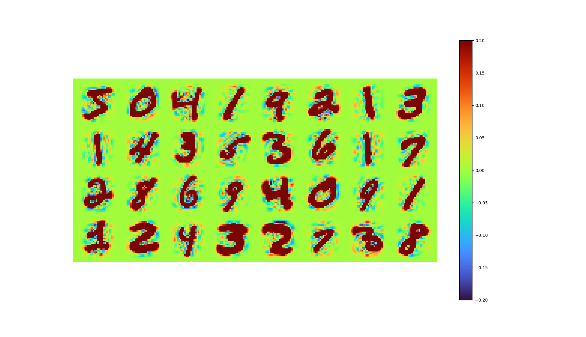
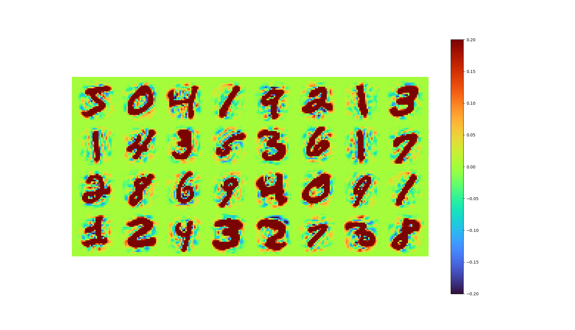
The MNIST handwritten digits dataset contains 70,000 (60,000 training, 1000 testing) greyscale fixed-size (28 * 28) images and is a standard dataset for benchmarking computer vision and deep learning algorithms.
![First 32 MNIST training set images, two-value images (0 or 1) are rerendered with a color mapping ranging [-0.2,0.2], consistent to the color mapping below](/2022/11/02/Autoencoder-identical-to-POD/MNIST original.png)
import torch
from torchvision import datasets, transforms, utils
import matplotlib.pyplot as plt
import numpy as np

# GPU if is available
device = torch.device("cuda:0" if torch.cuda.is_available() else "cpu")
# device = torch.device("mps" if torch.backends.mps.is_available() else "cpu")
print(device, " is in use")

# Load MNIST to a PyTorch Tensor
dataset = datasets.MNIST(root="./data",
                         train=True,
                         download=False,
                         transform=transforms.ToTensor())
POD result
In order to run POD , the training set is flattened, scaled to range [0,1] then centred by subtracting the mean image, resulting a data matrix \(\mathbf{X}\in\mathbb{R}^{784\times60000}\)
# Flatten from [60000, 28, 28] to [28*28, 60000], move to gpu
flatten_data = dataset.data.reshape(dataset.data.shape[0], -1).type(torch.FloatTensor)/255
mean_data = flatten_data.mean(axis=0)
flatten_data = flatten_data - mean_data
flatten_data = flatten_data.T.to(device)
The PyTorch SVD API is used for extracting POD modes, and the first 81 modes are selected to recover the data
# SVD and truncation
U, S, V = torch.svd(flatten_data)
k = 81
Uk = U[:, :k] # pod modes
Sk = torch.diag(S[:k]) # energy
Vk = V[:, :k]
The memory requirements for direct SVD are high on a dataset of this size. For larger data, such a direct approach is not practical.
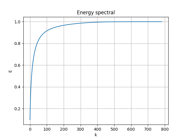
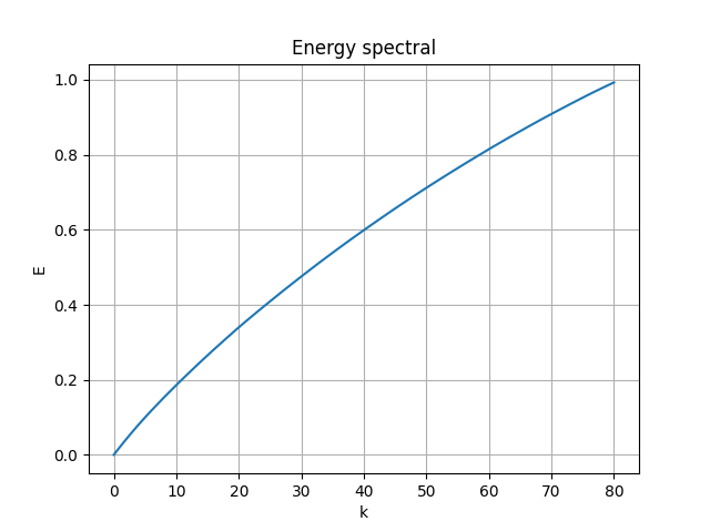
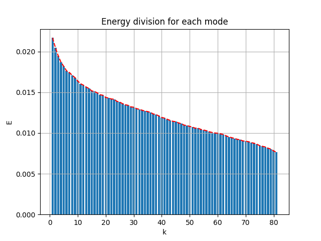
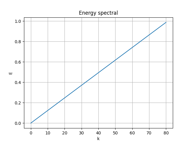
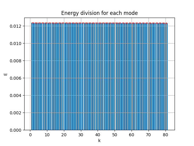
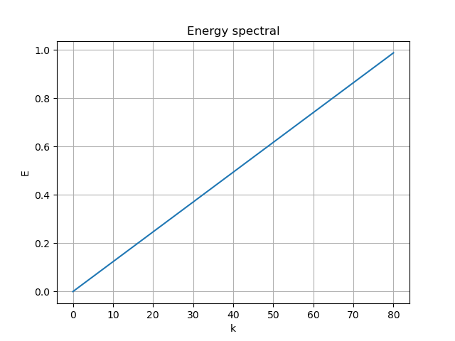
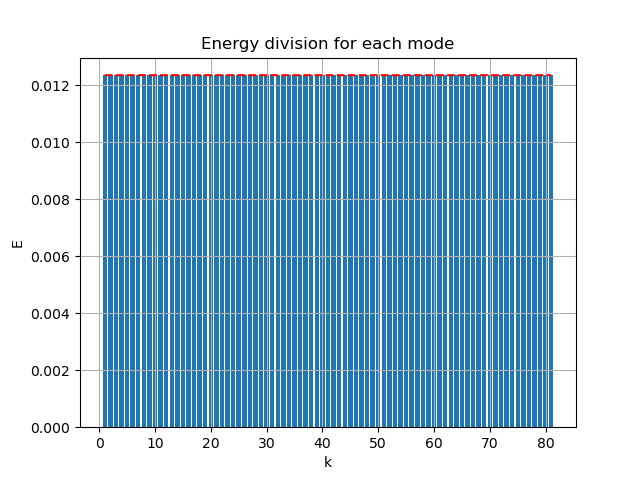
The energy spectral/division of each mode are shown below:
 |
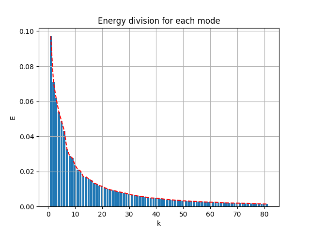 |
- the first 81 modes (in use) captured 89.2% of the total energy
- the first 87 modes captured 90% of the energy
- the first 331 modes captured 99% of the energy
Estimated data can be reconstructed from the extracted modes and associated weights. The error can be therefore calculated by the \(L2\) norm.
reconstructed = Uk@Sk@Vk.T
print("MSE loss", torch.square(reconstructed - flatten_data).mean().cpu().numpy())| SVD reconstructed | Error |
|---|---|
 |
 |
- the MSE error is 0.007265054
- pixel-to-pixel difference ranges from -0.997 to 0.920
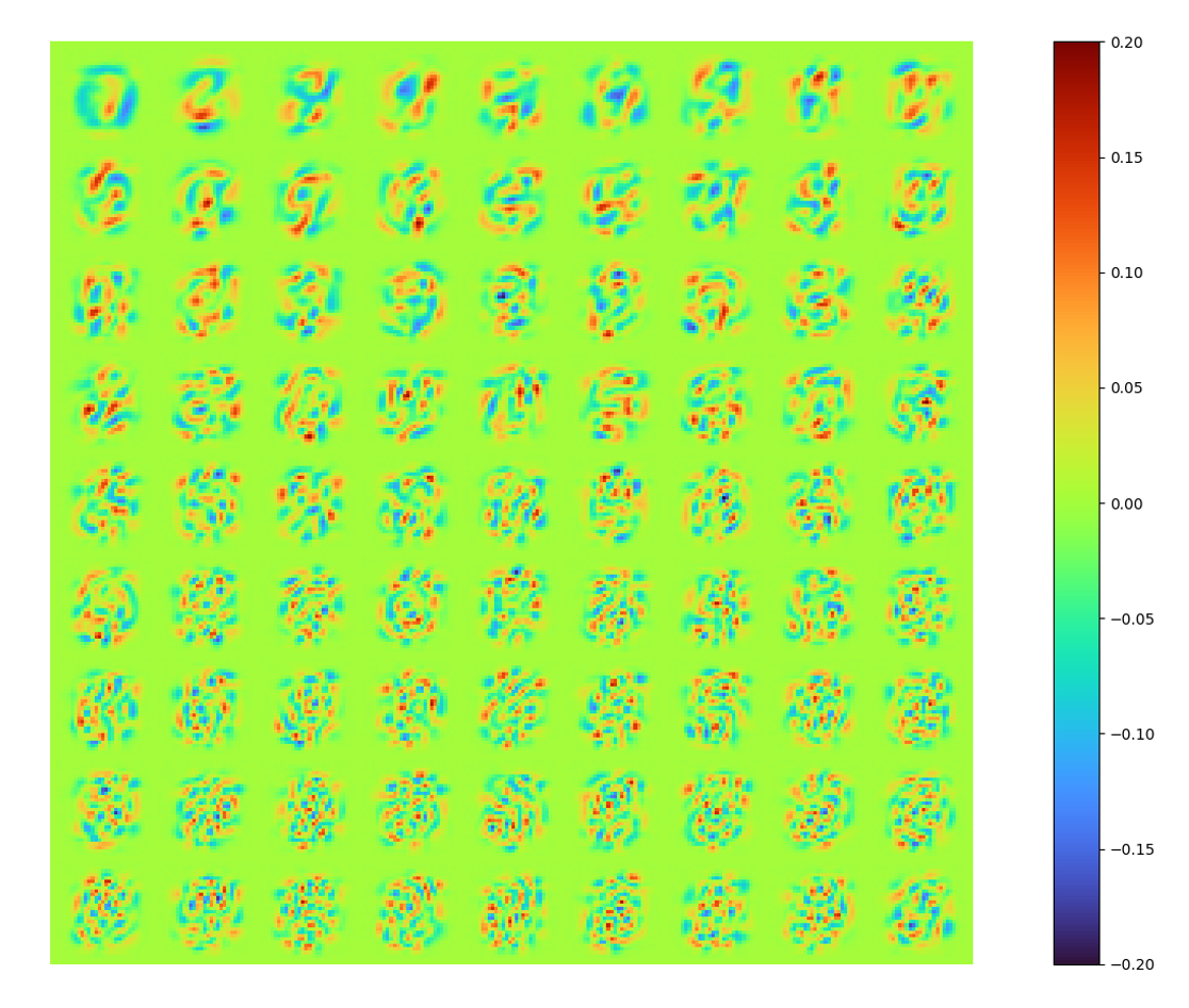
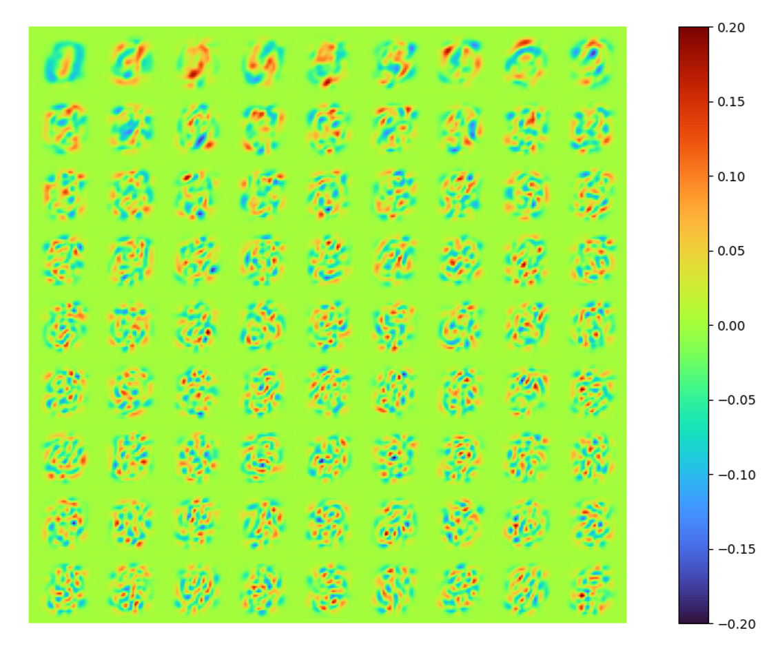
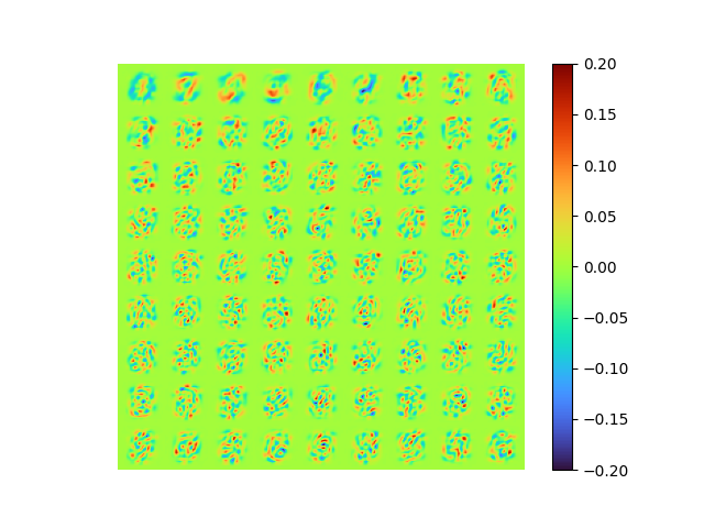
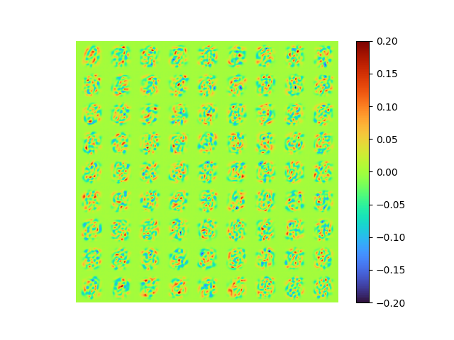
Note in this case, the color mapping ranges are all set to be [-0.2, 0.2] for consistence.
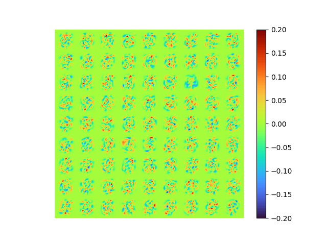
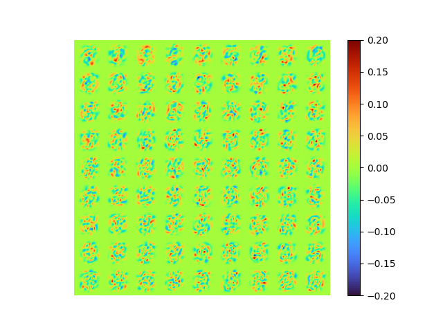
The modes can also be extracted easily. Note that these modes are orthonormal.
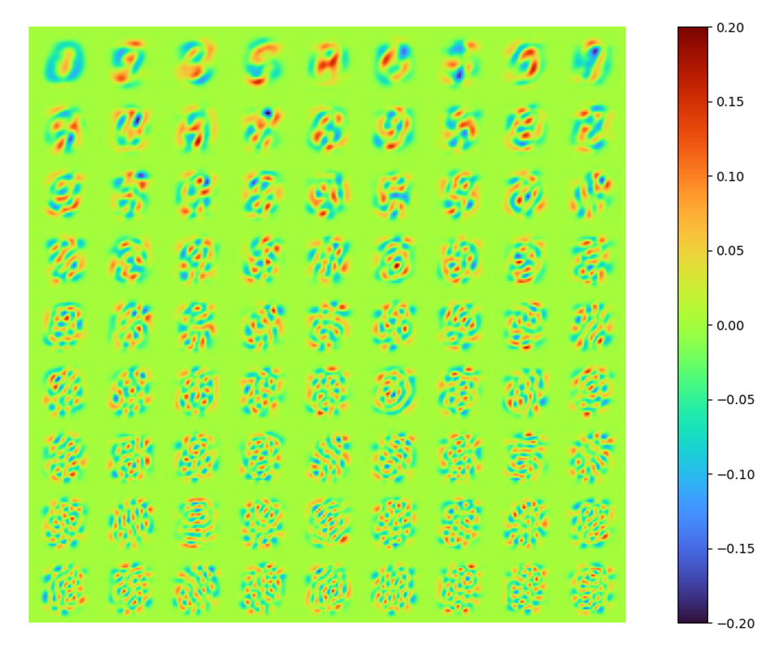
LAE results
The straightforward method is adopted, otherwise the size of weights is too large. The architecture is therefore:
from torchinfo import summary
# ...

k = 81

# Creating a AE class
# 28*28 ==> k ==> 28*28
class AE(torch.nn.Module):

    def __init__(self):
        super().__init__()
        self.encoder = torch.nn.Sequential(torch.nn.Linear(flatten_data.shape[1], k, bias=False))
        self.decoder = torch.nn.Sequential(torch.nn.Linear(k, flatten_data.shape[1], bias=False))

    def forward(self, x):
        encoded = self.encoder(x)
        decoded = self.decoder(encoded)
        return encoded, decoded

# Loss function and optimizer
loss_function = torch.nn.MSELoss()
optimizer = torch.optim.Adam(model.parameters(), lr=0.005)

# Summary
summary(model, input_size=(60000, 784))
==========================================================================================
Layer (type:depth-idx) Output Shape Param #
==========================================================================================
AE [60000, 81] --
├─Sequential: 1-1 [60000, 81] --
│ └─Linear: 2-1 [60000, 81] 63,504
├─Sequential: 1-2 [60000, 784] --
│ └─Linear: 2-2 [60000, 784] 63,504
==========================================================================================
Total params: 127,008
Trainable params: 127,008
Non-trainable params: 0
Total mult-adds (G): 7.62
==========================================================================================
Input size (MB): 188.16
Forward/backward pass size (MB): 415.20
Params size (MB): 0.51
Estimated Total Size (MB): 603.87
==========================================================================================An iterative mini batch training is implemented with batch_size = 25, epochs = 3.
The data reconstructed by LAE and the error of it are shown below.
| LAE Reconstructed | Error |
|---|---|
 |
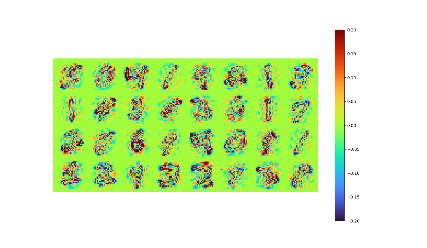 |
- MSE loss 0.00777
- pixel-to-pixel error ranges from -1.01 to 0.938
Note the optimal least error (error of POD) is not possible to reach because of nature of mini-batch regression.
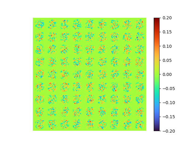
The set of mode is obtained by:
modes = np.array(model.decoder[0].weight.data.cpu())| raw modes | [method 1] error 0.00777 |
|---|---|
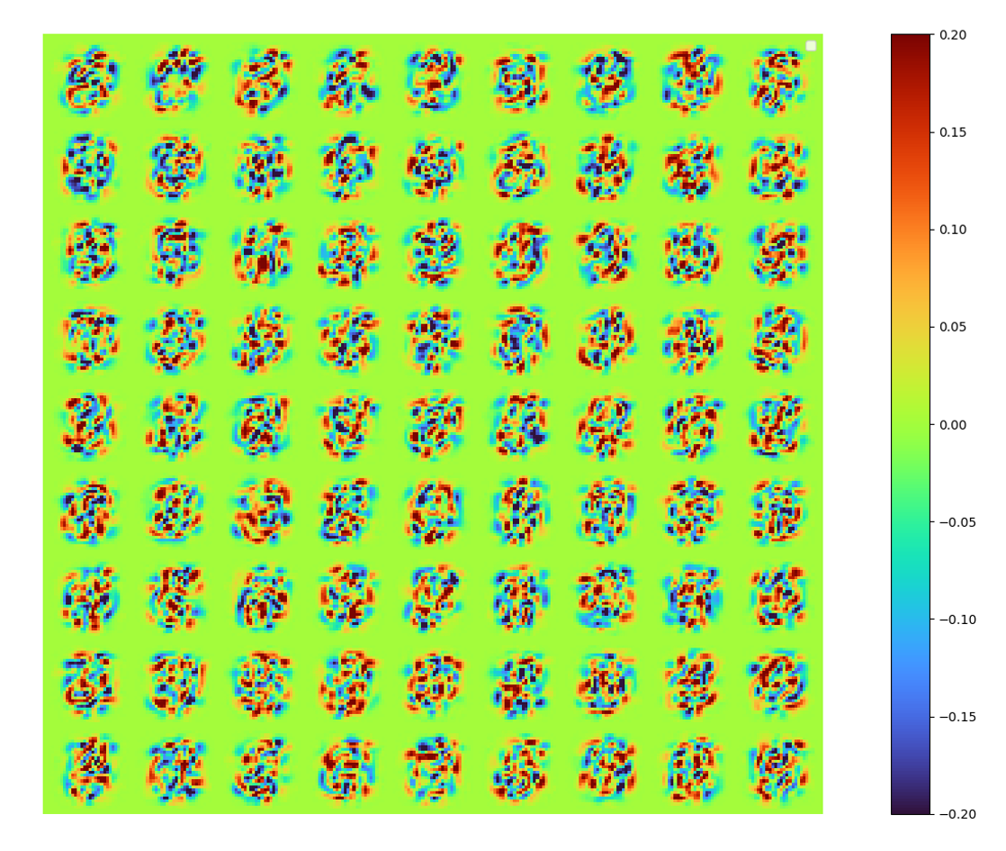 |
 |
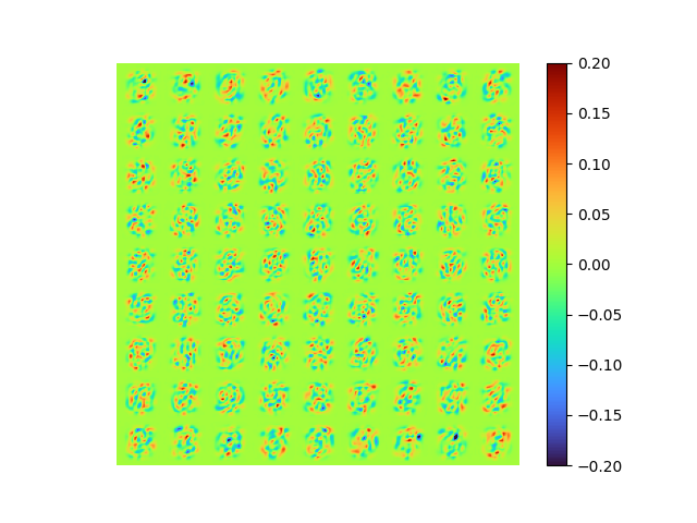
[method 1]
The raw modes constructed by LAE is obviously not identical to that of POD, in order to show the new spaces spanned by these two set of modes are identical/similar, orthonormalized the LAE modes by SVD, we can also get energy spectral (below) and a orthonormalized set of modes (above).
 |
 |
The singular values of each orthonormalized mode are more similar to each other, implying the orthogonality of the raw modes extracted by LAE is stronger, but still far from orthogonal.
The orthonormalized modes are, well, not quite same to that extracted by POD. So we do a small scale convergence check, taking some tricks (bigger batch size, learning rate scheduler etc) to have a better reconstruction result with MSE loss 0.0072723706, applying the similar process to get a orthonormalized set of modes.
| [method 1] error 0.007272370 | SVD, error 0.007265054 |
|---|---|
 |
|
The better equivalence (at least in terms of the first 2 modes) indicating the space spanned by LAE converges to that spanned by POD modes.
[method 2]
In order to apply orthogonal weights, first initialize the weight with radom orthogonal data.
from scipy.stats import ortho_group
# define flatten data, LAE, k = 81
model.encoder[0].weight = nn.Parameter(torch.tensor(ortho_group.rvs(dim=flatten_data.shape[0])[:,:k].T).float())
model.decoder[0].weight = nn.Parameter(torch.tensor(ortho_group.rvs(dim=flatten_data.shape[0])[:,:k]).float())
Then add another orthogonal losses to the MSE loss function
ortho_lambd = 0.01
# in the iteration loop:
  loss_ortho_de = torch.square(torch.dist(model.decoder[0].weight.T @ model.decoder[0].weight, torch.eye(k).to(device)))
  loss_ortho_en = torch.square(torch.dist(model.encoder[0].weight @ model.encoder[0].weight.T, torch.eye(k).to(device)))
  loss = loss_function(reconstructed, image) + ortho_lambd*(loss_ortho_de+loss_ortho_en)
The resulting modes and the singular value energy division is:
 |
 |
| [method 2] raw error 0.007268394 | [method 1] of [method 2] |
|---|---|
 |
 |
- MSE loss 0.007268394
- pixel-to-pixel error ranges from -0.99917483 to 0.91432786
The modes is nearly orthogonal yet it needs a good fine tuning of \(\lambda_{ortho}\) to balance the MSE error with the orthogonality error.
Neither the raw [method 2] modes nor the SVD orthogonalized modes associated to the POD modes, we will talk about that soon later.
[method 3]
Take advantage of the torch.nn.utils.parametrizations.orthogonal library, when define the LAE:
class AE(torch.nn.Module):

    def __init__(self):
        super().__init__()
+ 			self.encoder = torch.nn.Sequential(torch.nn.utils.parametrizations.orthogonal(torch.nn.Linear(flatten_data.shape[1], k, bias=False)))
+ 			self.decoder = torch.nn.Sequential(torch.nn.utils.parametrizations.orthogonal(torch.nn.Linear(k, flatten_data.shape[1], bias=False)))
- 			self.encoder = torch.nn.Sequential(torch.nn.Linear(flatten_data.shape[1], k, bias=False))
- 			self.decoder = torch.nn.Sequential(torch.nn.Linear(k, flatten_data.shape[1], bias=False))

    def forward(self, x):
        encoded = self.encoder(x)
        decoded = self.decoder(encoded)
        return encoded, decoded
The the singular value energy division and resulting modes are:
 |
 |
| [method 3] raw error 0.0072978497 | [method 1] of [method 3] |
|---|---|
 |
 |
- MSE loss 0.0072978497
- pixel-to-pixel error ranges from -0.9987151 to 0.9268836
The modes is perfect orthogonal, the loss is also small.
But the [method 2,3] modes are totally different from the POD modes. Because there is no regulation of the singular value of the modes, i.e. the optimality is not guaranteed.
[method 4] ( best )
Writing a custom parameterization class and apply to the decoder weights as:
class Svd_W_de(nn.Module):
    def forward(self, W2):
        U,_,_ = torch.svd(W2)
        return U

torch.nn.utils.parametrizations.parametrize.register_parametrization(model.decoder[0], "weight", Svd_W_de())
Tailer the network as
class AE(torch.nn.Module):

    def __init__(self):
        super().__init__()
        self.encoder = torch.nn.Sequential(torch.nn.utils.parametrizations.orthogonal(torch.nn.Linear(flatten_data.shape[1], k, bias=False)))
        self.decoder = torch.nn.Sequential(torch.nn.Linear(k, flatten_data.shape[1], bias=False))

    def forward(self, x):
        encoded = self.encoder(x)
+      	_,S,V = torch.svd(self.decoder[0].parametrizations.weight.original)
+       encoded = encoded@V@torch.diag(S)
        decoded = self.decoder(encoded)
        return encoded, decoded
The results are:
 |
 |
| [method 4] raw error 0.007290172 | [method 1] of [method 4] |
|---|---|
 |
 |
- MSE loss 0.007290172
- pixel-to-pixel error ranges from -1.005479 to 0.9235858
Great! The result is guaranteed as orthogonal and optimal, the error is small, and the model is end-to-end.
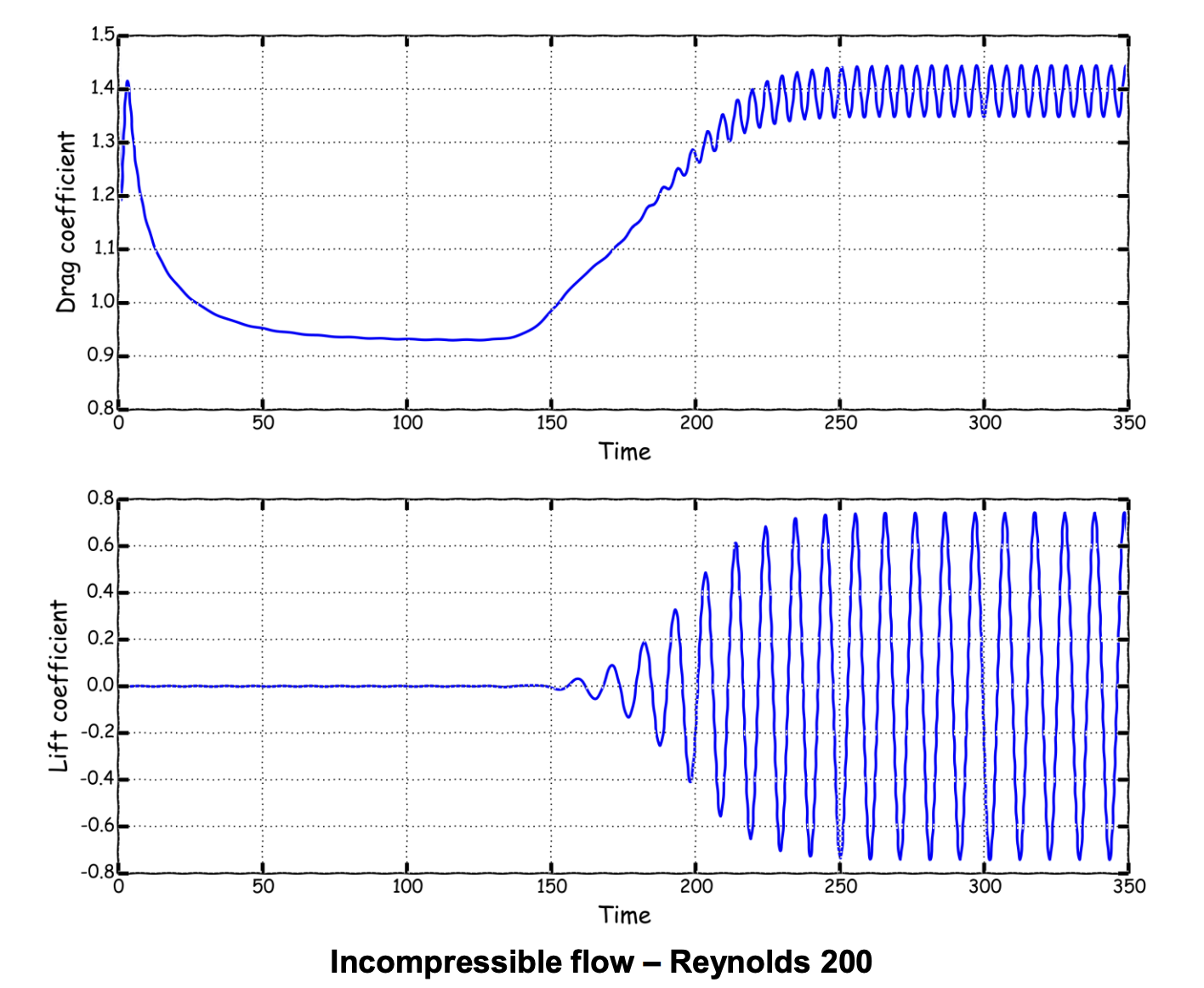
Flow past a cylinder
Flow over a 2D cylinder is the fundamental flow that captures the essential features of bluff-body flows. The periodic nature of it known as the von Kármán vortex shedding at Re>47 is always treated as an attractive initial test bed for decomposition methods. The POD result of the DNS simulation snapshots at Re=100 is shown below, the first 8 modes captures 99.97% of the flow fluctuations in terms of the KE.[3].
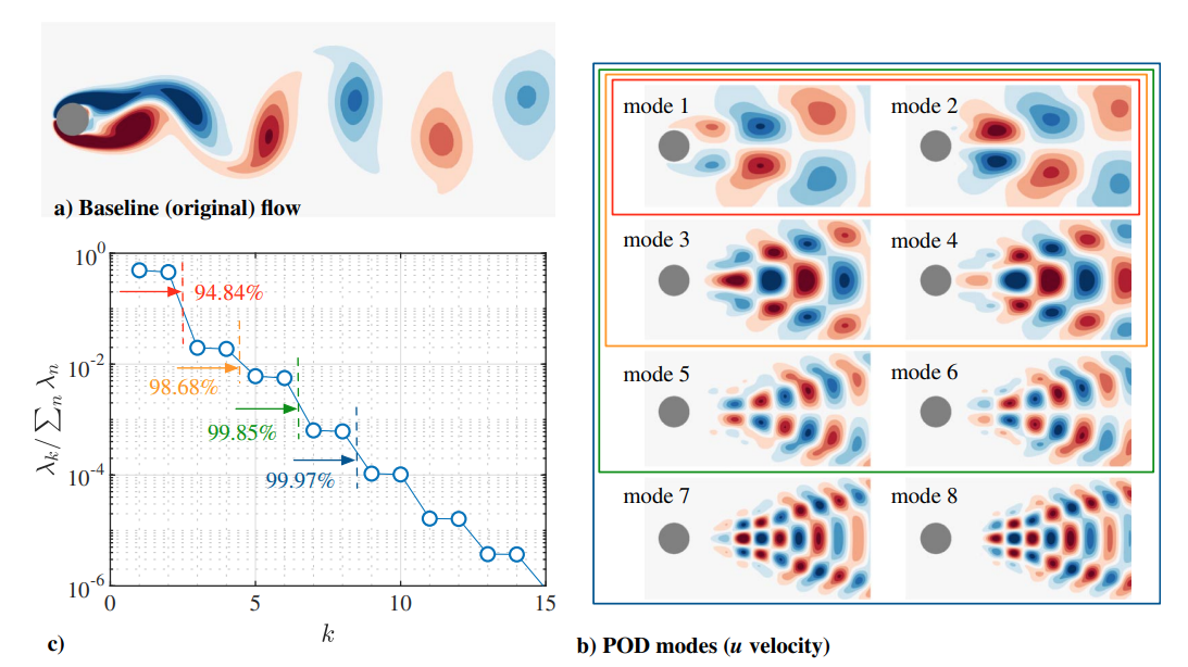
Note that these modes appear in pairs because of the periodical flow field and the real value nature of POD modes. Also note that the first two dominant modes are top-down asymmetry, associated with the asymmetry of the flow field.
Compared with dynamic mode decomposition (DMD), 2 POD modes in a pair are concluded by the real and imaginary parts of only one complex DMD mode. In another words, the 1st, 3rd, 5th, and the 2nd, 4th, 6th POD modes are identical with the real parts and imaginary parts of the 1st, 2nd, 3rd DMD modes respectively. (only true for exact periodical flow like this case)
For simplicity, here we take an unsteady FVM result at Re=200, from wolfdynamics OpenFOAM turtorial and perform POD and LAE decomposition based on the snapshots of velocity field from time 250 to 350. The resulting data matrix \(\mathbf{X}\in\mathbb{R}^{192080 \times 101}\)
 |
 |
# Load the fluid Dataset, flattened from [392, 490, 351] to [192080, 351]
flatten_data = load_img_as_matrix("./data/cylinder")
mean_data = flatten_data[250:,:].mean(axis=0)
flatten_data = flatten_data - mean_data
flatten_data = torch.tensor(flatten_data.T[:,250:])
POD result
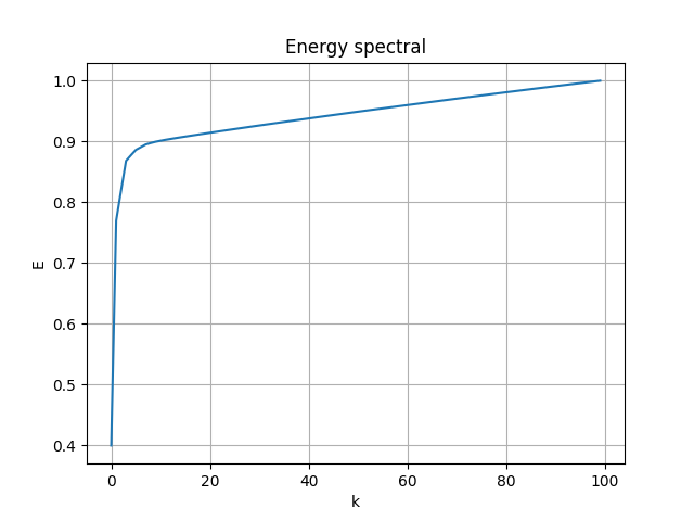
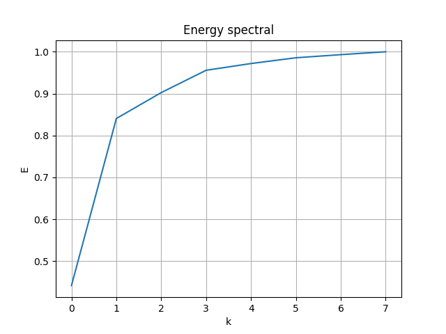
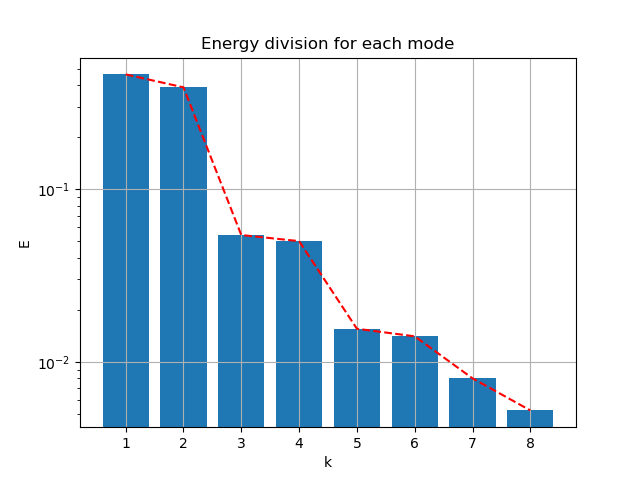
Follow the process of last case, the energy spectral/division of each mode:
 |
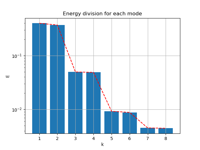 |
- First 2 modes capture 76.95% of energy
- First 4 modes capture 86.81% of energy
- First 6 modes capture 88.61% of energy
- First 8 modes capture 89.51%of energy
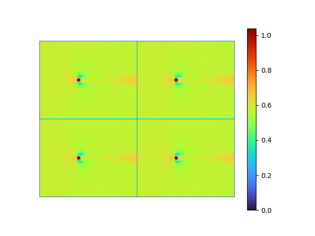
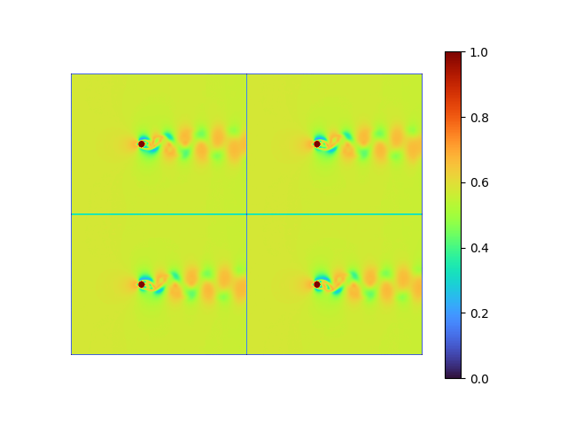
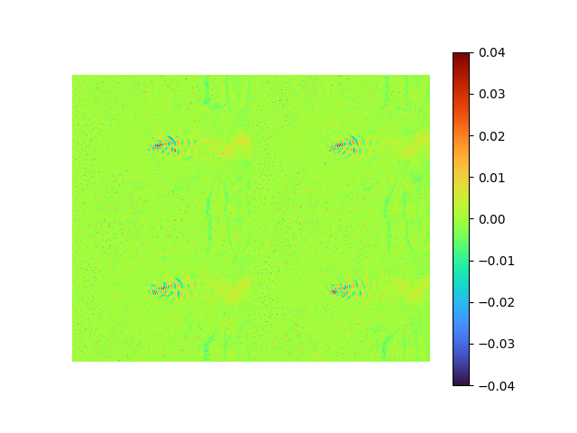
And the original, reconstructed, error results are
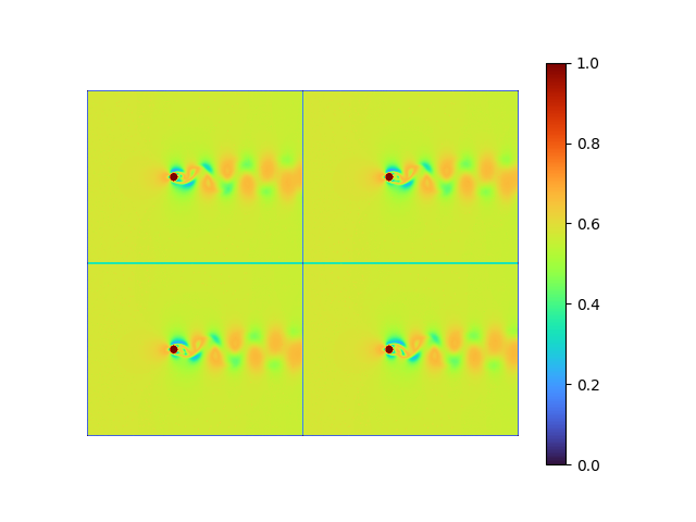 |
 |
 |
- MSE loss 7.4397925e-05
- pixel-to-pixel error ranges from -0.1370289 to 0.12152482
The first 8 dominant POD modes are shown bleow:
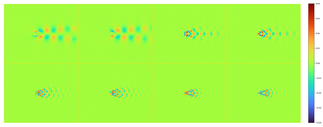
Note the modes looks very similar to the standard result at the beginning of this case at Re = 100.
LAE results
Straightforward ( FAILED )
With straightforward method, it is really difficult for autoencoder to converge, and the model is prone to gradient vanishing because of the big data size compared with the length of data.
print("shape of dataset:", flatten_data.shape)
summary(model, input_size=(101, 192080))
print("encoder weight shape: ", model.encoder[0].weight.shape)
print("decoder weight shape: ", model.decoder[0].weight.shape)
shape of dataset: torch.Size([101, 192080])
==========================================================================================
Layer (type:depth-idx) Output Shape Param #
==========================================================================================
AE [101, 8] --
├─Sequential: 1-1 [101, 8] --
│ └─Linear: 2-1 [101, 8] 1,536,640
├─Sequential: 1-2 [101, 192080] --
│ └─Linear: 2-2 [101, 192080] 1,536,640
==========================================================================================
Total params: 3,073,280
Trainable params: 3,073,280
Non-trainable params: 0
Total mult-adds (M): 310.40
==========================================================================================
Input size (MB): 77.60
Forward/backward pass size (MB): 155.21
Params size (MB): 12.29
Estimated Total Size (MB): 245.10
==========================================================================================
encoder weight shape: torch.Size([8, 192080])
decoder weight shape: torch.Size([192080, 8])| reconstructed | error | raw modes | [method 1] |
|---|---|---|---|
 |
 |
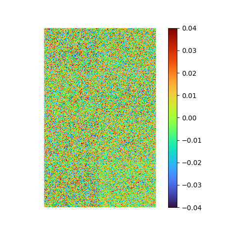 |
![[method 1] orthogonalized strightforward AE modes](/2022/11/02/Autoencoder-identical-to-POD/SVD AE st first 8 modes extracted from fluid - mean.png) |
The fluid data FAILs being recovered, the repetitive pattern shown on the recovered images is the mean flow.
Compared the recovered orthonormal modes extracted by straightforward AE with POD modes, only the first dominant POD mode is barely captured with low amplitude (note the data range difference), indicating a gradient vanishing.
Transposition [method 1]
To take advantage of the better performance of neural network on large data length, and to prevent the overfitting and gradient vanishing, transpose the flattened data and make LAE compress it in terms of the data length dimension. (101 -> 8 -> 101)
+  flatten_data = flatten_data.T
print("shape of dataset:", flatten_data.shape)
- summary(model, input_size=(101, 192080))
+ summary(model, input_size=(192080, 101))
print("encoder weight shape: ", model.encoder[0].weight.shape)
print("decoder weight shape: ", model.decoder[0].weight.shape)
shape of dataset: torch.Size([192080, 101])
==========================================================================================
Layer (type:depth-idx) Output Shape Param #
==========================================================================================
AE [192080, 8] --
├─Sequential: 1-1 [192080, 8] --
│ └─Linear: 2-1 [192080, 8] 808
├─Sequential: 1-2 [192080, 101] --
│ └─Linear: 2-2 [192080, 101] 808
==========================================================================================
Total params: 1,616
Trainable params: 1,616
Non-trainable params: 0
Total mult-adds (M): 310.40
==========================================================================================
Input size (MB): 77.60
Forward/backward pass size (MB): 167.49
Params size (MB): 0.01
Estimated Total Size (MB): 245.10
==========================================================================================
encoder weight shape: torch.Size([8, 101])
decoder weight shape: torch.Size([101, 8])This autoencoder can be well trained in seconds, and the reconstruction and error result are:
 |
 |
- MSE loss 7.4815114e-05
- pixel-to-pixel error ranges from -0.13534062 to 0.12123385
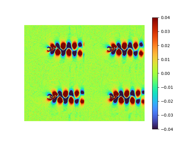
The first 8 modes and [method 1] normalized modes extracted by LAE are:
| energy | raw modes | [method 1] error 7.4815114e-05 |
|---|---|---|
  |
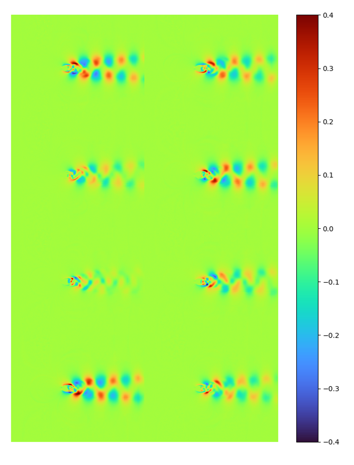 |
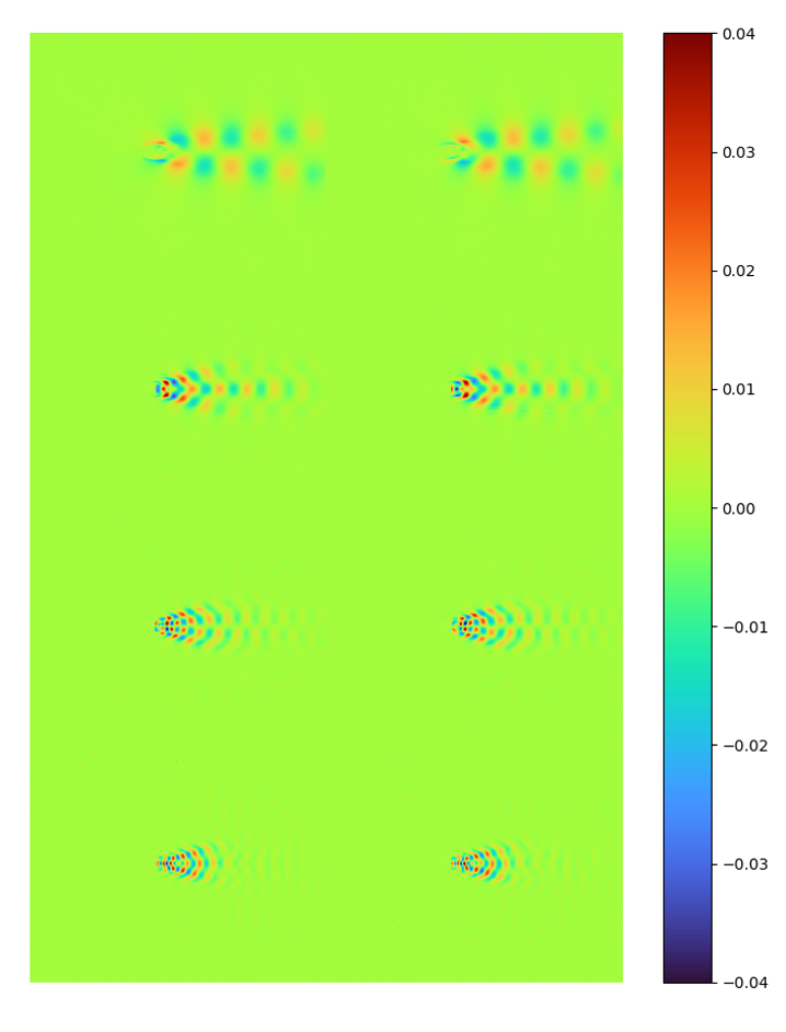 |
It can be seen that the latent space spanned by LAE modes and POD are nearly identical.
Note the data range for the raw mode is different (-0.4~0.4 instead of -0.04~0.04)
[method 5] ( FAILED )
The easiest way is applying SVD to the bottleneck feature every step as:
class AE(torch.nn.Module):

    def __init__(self):
        super().__init__()
        self.encoder = torch.nn.Sequential(torch.nn.Linear(flatten_data.shape[1], k, bias=False))
        self.decoder = torch.nn.Sequential(torch.nn.Linear(k, flatten_data.shape[1], bias=False))

    def forward(self, x):
        encoded = self.encoder(x)
+       svd_encoded,_,_ = torch.svd(encoded)
        decoded = self.decoder(encoded)
-       return encoded, decoded
+       return svd_encoded, decoded
This operation has no advantage but 3 drawbacks:
- Exactly identical to the result of
[method 1]in full batch training. But the resulting mode is wrong with mini-batch gradient descend. - This operation does not affect the training process.
- It is computational heavier than
[method 1]as the latter only requires one singular value decomposition step
Another way is to pass the \(\mathbf{U}\) (svd_encoded) to the decoder and multiplying the weight by \(\boldsymbol{\Sigma}\mathbf{V^T}\), mimicking [method 4].
class AE(torch.nn.Module):

    def __init__(self):
        super().__init__()
        self.encoder = torch.nn.Sequential(torch.nn.Linear(flatten_data.shape[1], k, bias=False))
        self.decoder = torch.nn.Sequential(torch.nn.Linear(k, flatten_data.shape[1], bias=False))
        self.SVT = torch.zeros((k,k))

    def forward(self, x):
        encoded = self.encoder(x)
        svd_encoded,S,V = torch.svd(encoded)
        decoded = self.decoder(svd_encoded)
        self.SVT = V@torch.diag(S)
        return svd_encoded, decoded


class Svd_W_de(nn.Module):
    def __init__(self, SVT):
        super().__init__()
        self.SVT = SVT
    def forward(self, X):
        return X.to(device)@self.SVT.to(device)


# Model Initialization
model = AE()
torch.nn.utils.parametrizations.parametrize.register_parametrization(model.decoder[0], "weight", Svd_W_de(model.SVT))
This operation has no advantage but 2 vital drawbacks:
- Cannot be trained
- The resulting mode is wrong with mini-batch gradient descend
As a result, [method 5] is therefore deprecated.
Conclusion
When to use linear autoencoder?
When data is big, the latent space can be well captured with a much lower memory requirement.
When offline training is impractical, for example when new data coming through constantly.
The relationship between LAE and POD modes?
There is no regulation to the form of LAE modes while the POD modes are orthonormal which is suitable to design a sparse representation.
The latent space captured by LAE converges to the optimal space spanned by POD modes.
Straightforward vs transposition LAE?
It mainly depends on the aspect ratio of input data. In order to decrease the number of weights/parameters, it is better to choose a type such that the longer dimension of data is preserved.
- Straightforward method suitable for very wide data, like MNIST.
- Transposition method for very thin data like flow velocity snapshots.
- If a multi-layer non-linear Autoencoder is applied, the modes extracted by the transposed AE are still easy to get access
Conclusion on the improvement methods?
[method1] [method2] [method3] [method4] [method5] note suitable LAE both straightforward straightforward straightforward transposition end-to-end ❌ ✅ ✅ ✅ ✅ orthogonality of the modes perfect nearly perfect perfect perfect perfect optimality ✅ ❌ ❌ ✅ ❌ converge to the POD modes ✅ ❌ ❌ ✅ ❌ reconstruction error (straightforward) 7.272e-3 7.268e-3 7.298e-3 7.290e-3 NAN POD error
7.265e-3reconstruction error (transposition) 7.48e-5 NAN NAN NAN 7.03e-4 POD error
7.44e-05
Appendix
Ablation test of L2 regularization of LAE on MNIST
Different weight decay and learning rate are applied, and the raw modes are inspected by [method 1].
For learning rate \(\alpha = 0.005\), the energy spectral and division for weight decay \(\lambda\) from \(0.005\) to \(0\) are plotted animately as below:
 |
 |
and the raw modes and orthogonal modes recovered by [method 1] are shown below:
 |
 |
The MSE error and the range of the mode value is plotted with the weight decay and learning rate as well:
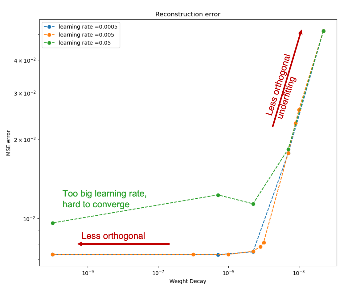 |
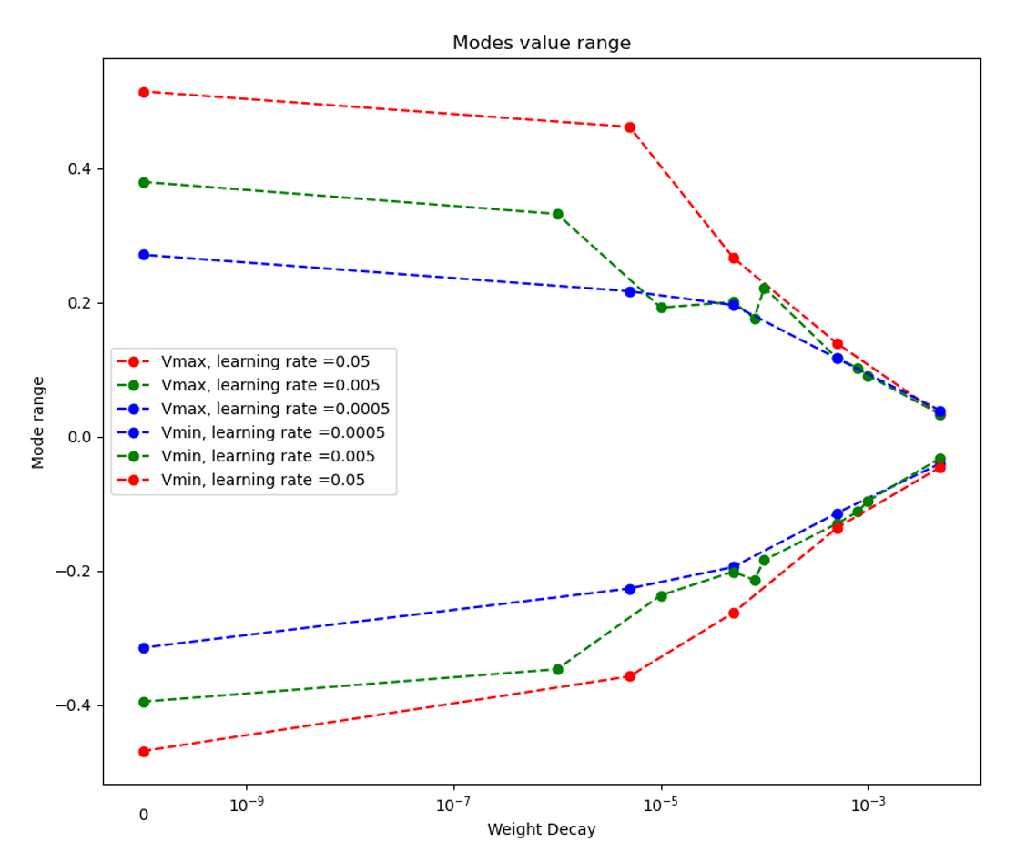 |
As we can see, learning rate does not affect the mean square error, but the range of the mode value. And weight decay can be used to control the modes' orthogonality, a suitable weight decay for example \(8e-5\) results in a better orthogonality and the recovered modes (shown below)· shows a better resemblance of the POD modes.
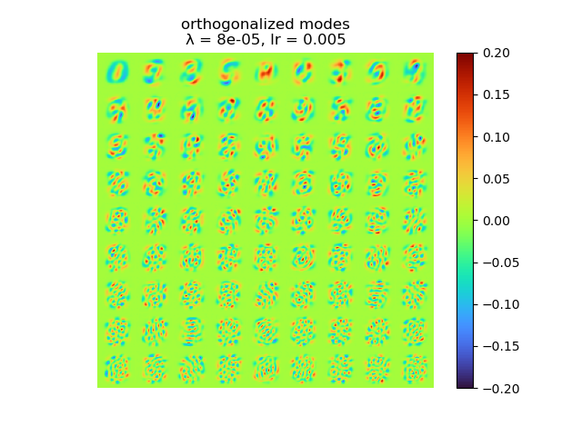 |
|
Besides, it is interesting to see that although the biggest weight decay \(0.005\) fail to recover most of the modes, the raw modes are very similar to the its recovered modes, like a shuffled version of many copies of the recovered modes regardless the magnitude difference.
 |
 |
References
- Milano, M., & Koumoutsakos, P. (2002). Neural network modeling for near wall turbulent flow. Journal of Computational Physics, 182(1), 1-26. ↩︎
- Brunton, S. L., Noack, B. R., & Koumoutsakos, P. (2020). Machine learning for fluid mechanics. Annual review of fluid mechanics, 52, 477-508. ↩︎
- Taira, K., Hemati, M. S., Brunton, S. L., Sun, Y., Duraisamy, K., Bagheri, S., ... & Yeh, C. A. (2020). Modal analysis of fluid flows: Applications and outlook. AIAA journal, 58(3), 998-1022. ↩︎
- Brock, A., Lim, T., Ritchie, J. M., & Weston, N. (2016). Neural photo editing with introspective adversarial networks. arXiv preprint arXiv:1609.07093. ↩︎
- Brock, A., Donahue, J., & Simonyan, K. (2018). Large scale GAN training for high fidelity natural image synthesis. arXiv preprint arXiv:1809.11096. ↩︎
- Lubana, E. S., Trivedi, P., Hougen, C., Dick, R. P., & Hero, A. O. (2020). OrthoReg: Robust Network Pruning Using Orthonormality Regularization. arXiv preprint arXiv:2009.05014. ↩︎
- Blalock, D., Gonzalez Ortiz, J. J., Frankle, J., & Guttag, J. (2020). What is the state of neural network pruning?. Proceedings of machine learning and systems, 2, 129-146. ↩︎