RANS recap

Attend to validate a turbulence modeling, need a quick recap on the classical theorem.

This is a crash introduction of turbulence and RANs, if need further information, here are some useful references. Most of the concepts, formulas, figures of this blog are collected from these resources:

note: Viscous Flows and Turbulence - profs.scienze.univr.it

slides: Turbulence modeling in OpenFOAM and general CFD - Advanced training

video: Turbulence Closure Models: Reynolds Averaged Navier Stokes (RANS) & Large Eddy Simulations (LES)

book: The structure of turbulent shear flow ^[7]

Turbulence Introduction

The Nature of Turbulent Flow

Turbulent flow is characterised by:

1. Three-dimensionality. Turbulence is inherently three-dimensional. Although some people study two-dimensional turbulence (this may have some application to geophysical flows (see figure 6.1). Note that the “stretching and tilting” term in the vorticity transport equation is absent in two-dimensional flows, and therefore two-dimensional turbulence is considerably simpler than the real-life three-dimensional variety.

2. Time-dependency. Turbulence is characterised by unsteady variations in velocity, density, temperature or concentration, and the variation (fluctuations) occurs over a wide range of time scales. Turbulence has a broad frequency spectrum.

3. A wide range of length scales. Turbulence has a broad wavenumber spectrum. If we consider the example of turbulent pipe flow, a range of scales which goes from the largest (of order \(D\), the pipe diameter) to the smallest (of order \(ν/u_\tau\), where \(u_\tau\) is the friction velocity, which is a velocity scale based on the wall shear stress: it is of the same order as a typical velocity fluctuation)

4. Effective mixing of all fluid properties.

Study Turbulence

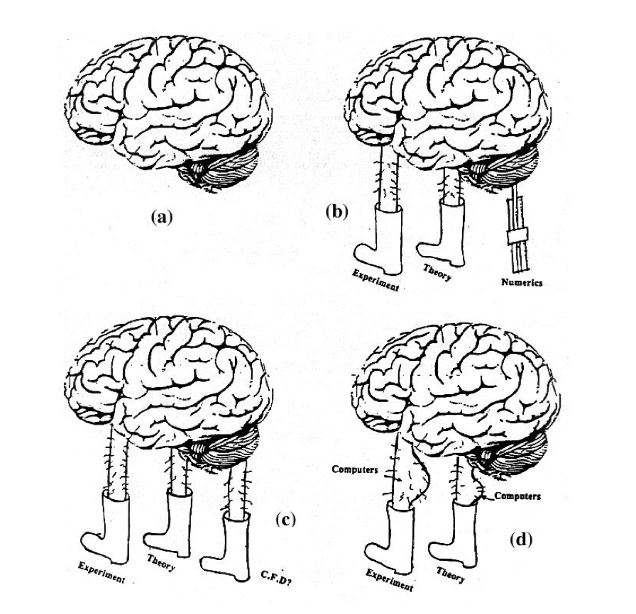
Historically, studies of turbulence have relied on a very restricted set of “tools”:

1. Approximate analysis of average properties of highly idealized turbulent flows (eg. grid turbulence);
2. Analysis of idealized linear stability problems;
3. Measurements of time-averaged properties and ensemble-average properties (\(\bar{U}, \bar{U'^2}, \bar{U'v'}, \Psi(\omega), p(u)\), etc.);
4. Flow visualization;
5. Dimensional analysis and scaling arguments.

From this work we have obtained

1. a small set of widely accepted “facts”, for example, the logarithmic variation of velocity in a turbulent boundary layer;
2. a small set of widely accepted correlations, for example the friction factor for pipes as a function of Reynolds number;
3. a small set of widely accepted theories eg. Kolmogoroff’s inertial range, Batchelor’s final decay of grid turbulence;
4. a qualitative notion of energy transfer (the energy cascade);
5. the kinematics and other general features of turbulence and eddies, for example the role of bulges, horshoe-vortices, “typical” eddies, etc.;
6. some useful but rather restricted sets of predictive tools, for example, the k-ε turbulence model;
7. a good appreciation of scaling arguments.

The difficulty is:

• Turbulence is complex. Extremely complex.

The main goal is:

• To develop approximations to the N-S equations which embody sufficient dynamical information to allow reliable and efficient predictions of turbulent flows.

We need:

1. high quality simulations;
2. high quality experiments;
3. good ideas.

Approaches to Turbulence

The major varieties are the

• time-averaged approach (also called Reynolds averaged approach);
• ensemble-averaged approach;
• instantaneous realisation approach

Reynolds-averaged

• most common approach
• most studied
• most limited in terms of understanding
• form the basis of all engineering calculation methods

idea

• turbulence is seen as a purely statistical phenomena
• N-S equations are written in terms of mean quantities by using time averages
• turbulence model is incorporated to close the model

Ensemble-averaged

• a way of thinking, rather than a parallel approach to RANs

idea

• turbulence has an underlying structure instead of randomness
• similarity among eddies, determine the average properties of an eddy, and how these properties scale with size, position, etc
• take some of the turbulent structure into account

Examples see phase-averaging (Cantwell & Coles^[1] Perry & Tan^[2]) and VITA^[3] approach (Spina & Donovan^[4]).

Instantaneous realisation

• a way of thinking, again
• one can do this in experiments (e.g. PIV (Particle-Image Velocimetry)) or simulations.

idea

• understand turbulence by looking at individual events
• picking out features which occur often (link to ensemble-averaged approach above)
• looking at a relatively small number of events

see Robinson's work^[5].

Note that these 3 approaches can be used together by researchers, there are no cut line among these.

What is structure in turbulence?

Turbulence usually displays departures from Gaussian behavior - these departures may be called structure, and might be embodied in terms of the moments of the pdf’s of \(u', v'\) and \(w'\)

A description of individual eddying motions in the turbulence. Also called coherent structures ” if they represent some sort of entity which can be followed in time.

Reynolds-Averaged Equations

Example: Turbulent channel flow

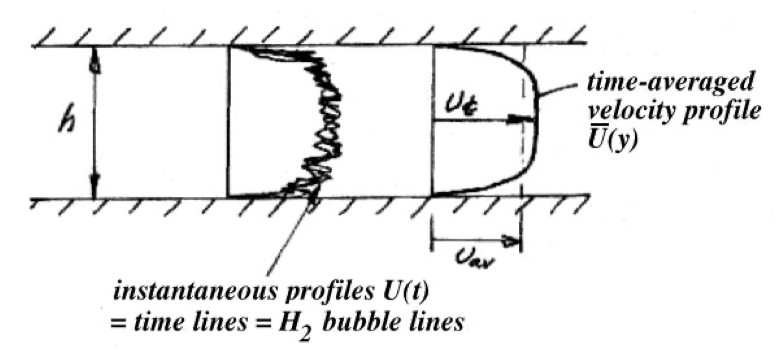
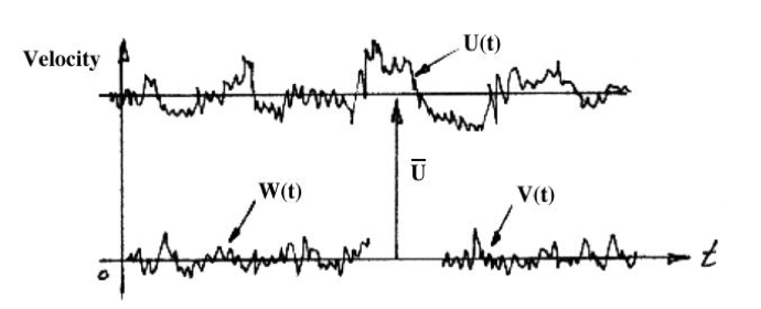
Consider the above channel flow at high Reynolds number ( \(Re >> 2000\), where \(Re = U_{av}h/\nu\) ). The pressure drop driving the flow is assumed to be steady. At any point in the flow, the magnitude of the velocity in all three directions fluctuates in time. If we insert a probe into the flow so that we can measure the velocity at a given point, we would see the time traces shown in the diagram. Note that we can define a time-averaged velocity: \[ \bar{U}(x)=\lim _{T \rightarrow \infty} \frac{1}{T} \int_{t_0}^{t_0+T} U(x, t) d t \] where \(t_0\) is an arbitrary start sampling time

and a space-averaged velocity: \[ U_{a v}=\frac{1}{A} \int \bar{U} d A=\frac{1}{h} \int_{-h / 2}^{+h / 2} \bar{U} d y . \]

Reynolds decomposition

The concept of a time-averaged velocity also leads to the concept of the flow being composed of a time-averaged field, and a fluctuating field. This is called the Reynolds decomposition where we write (in Cartesian coordinates, where \(\mathbf{V} = U\mathbf{i}+V\mathbf{j}+W\mathbf{k}\) ): \[ \color{purple} \begin{aligned} \mathbf{V}(\mathbf{x},t)=\bar{\mathbf{V}}(\mathbf{x})+\mathbf{v}'(\mathbf{x},t) \\ p(\mathbf{x},t)=\bar{p}(\mathbf{x})+p'(\mathbf{x},t) \end{aligned} \] (\(V, W\) and the pressure \(p\) are decomposed similarly)

The rules for averaging are: \[\begin{aligned}\overline{a^{\prime}} &=0 \\\overline{a+b} &=\bar{a}+\bar{b} \\\overline{\bar{a}} &=\bar{a} \\\overline{\bar{a} \cdot \bar{b}} &=\bar{a} \cdot \bar{b} \\\overline{\left( \frac{\partial a}{\partial s}\right)} &=\frac{\partial \bar{a}}{\partial s}\end{aligned}\] IMPORTANT: \[\color{purple}\overline{a \cdot b} \neq \bar{a}\bar{b}\] This means even though the fluctuation \(u_i'\) is zero mean i.e. \(\overline{u_i^{\prime}}=0\), it is NOT zero variance i.e. the higher motion (Reynolds stress) is non-trivial i.e. \[\begin{aligned}\overline{u'^2} &\neq 0 \\\overline{u^{\prime}v^{\prime}}& \neq 0\end{aligned}\]

Start with the continuity and Navier-Stokes equations (for incompressible flow and no body forces): \[ \begin{aligned} \nabla \cdot \mathbf{V}&=0 \\ \\ \frac{D \mathbf{V}}{D t}=\frac{\partial \mathbf{V}}{\partial t}+\mathbf{V} \cdot \nabla \mathbf{V}&=-\frac{1}{\rho} \nabla p+\nu \nabla^2 \mathbf{V} \\ or \quad \frac{\partial u_i}{\partial t}+u_i \frac{\partial u_i}{\partial x_j}&=-\frac{1}{\rho} \frac{\partial p}{\partial x_i}+\nu \frac{\partial^2 u_i}{\partial x_j^2} \end{aligned} \] Plug the Reynolds decomposition of \(\mathbf{V}\) into Continuity and Momentum:

Continuity Equation

With the Reynolds decomposition, the continuity equation becomes: \[ \frac{\partial \bar{U}}{\partial x}+\frac{\partial \bar{V}}{\partial y}+\frac{\partial \bar{W}}{\partial z}+\frac{\partial u^{\prime}}{\partial x}+\frac{\partial v^{\prime}}{\partial y}+\frac{\partial w^{\prime}}{\partial z}=0 \] Taking the time average we obtain: \[ \frac{\partial \bar{U}}{\partial x}+\frac{\partial \bar{V}}{\partial y}+\frac{\partial \bar{W}}{\partial z}=0 \] That is, \[ \color{purple} \nabla \cdot \overline{\mathbf{V}}=0 \]

Note that \(\nabla \cdot \mathbf{v}^{\prime}=0\) as well, denoting the mean and fluctuating velocities individually satisfy the continuity equation.

Momentum Equation

Consider the x-component of the momentum equation, just like decomposing the continuity equation \[ \begin{aligned} &\frac{\partial \bar{U}}{\partial t}+\frac{\partial u^{\prime}}{\partial t}\\ &+\bar{U} \frac{\partial \bar{U}}{\partial x}+u^{\prime} \frac{\partial u^{\prime}}{\partial x}+u^{\prime} \frac{\partial \bar{U}}{\partial x}+\bar{U} \frac{\partial u^{\prime}}{\partial x}\\ &+\bar{V} \frac{\partial \bar{U}}{\partial y}+v^{\prime} \frac{\partial u^{\prime}}{\partial y}+v^{\prime} \frac{\partial \bar{U}}{\partial y}+\bar{V} \frac{\partial u^{\prime}}{\partial y}\\ &+\bar{W} \frac{\partial \bar{U}}{\partial z}+w^{\prime} \frac{\partial u^{\prime}}{\partial z}+w^{\prime} \frac{\partial \bar{U}}{\partial z}+\bar{W} \frac{\partial u^{\prime}}{\partial z}\\ &=-\frac{1}{\rho} \frac{\partial \bar{p}}{\partial x}-\frac{1}{\rho} \frac{\partial p^{\prime}}{\partial x}+\nu \nabla^2 \bar{U}+\nu \nabla^2 u^{\prime} . \end{aligned} \] Taking the time average, we have \[ \begin{aligned} U \frac{\partial U}{\partial x}+V \frac{\partial U}{\partial y}+&W \frac{\partial U}{\partial z}=\\ -\frac{1}{\rho} &\frac{\partial p}{\partial x}+\nu \nabla^2 U -\left(\overline{u^{\prime}\frac{\partial u^{\prime}}{\partial x}}+\overline{v^{\prime}\frac{\partial u^{\prime}}{\partial x}}+\overline{v^{\prime}\frac{\partial u^{\prime}}{\partial x}}\right) \end{aligned} \]

Recall the knowledge of the chain rule, we can divided the last term with: \[\begin{aligned}& \overline{u^{\prime} u_x^{\prime}}=\frac{\partial \overline{u^{\prime} u^{\prime}}}{\partial x}-\overline{u^{\prime} u_x^{\prime}} \\&\overline{v^{\prime} u_y^{\prime}}=\frac{\partial \overline{u^{\prime} v^{\prime}}}{\partial y}-\overline{u^{\prime} v_y^{\prime}} \\&\overline{w^{\prime} u_z^{\prime}}=\frac{\partial \overline{u^{\prime} w^{\prime}}}{\partial z}-\overline{u^{\prime} w_z^{\prime}}\end{aligned}\]

cancel out the underlying continuity equation multiplied by \(u'\) term, we obtain: \[ \begin{aligned} U \frac{\partial U}{\partial x}+V \frac{\partial U}{\partial y}+&W \frac{\partial U}{\partial z}=\\ -\frac{1}{\rho} &\frac{\partial p}{\partial x}+\nu \nabla^2 U-\left(\frac{\partial \overline{u^{\prime 2}}}{\partial x}+\frac{\partial \overline{u^{\prime} v^{\prime}}}{\partial y}+\frac{\partial \overline{u^{\prime} w^{\prime}}}{\partial z} + \underbrace{u' \nabla \cdot \mathbf{v}^{\prime}}_{ = 0}\right) \end{aligned} \] Similarly, for the \(y\) and \(z\) components: \[ \begin{aligned} U \frac{\partial V}{\partial x}+V \frac{\partial V}{\partial y}+&W \frac{\partial V}{\partial z}= \\ -\frac{1}{\rho} &\frac{\partial p}{\partial y}+\nu \nabla^2 V -\left(\frac{\partial \overline{u^{\prime} v^{\prime}}}{\partial x}+\frac{\partial \overline{v^{\prime 2}}}{\partial y}+\frac{\partial \overline{v^{\prime} w^{\prime}}}{\partial z}\right)\\ \\ U \frac{\partial W}{\partial x}+V \frac{\partial W}{\partial y}+&W \frac{\partial W}{\partial z}= \\ -\frac{1}{\rho}& \frac{\partial p}{\partial z}+\nu \nabla^2 W-\left(\frac{\partial \overline{u^{\prime} w^{\prime}}}{\partial x}+\frac{\partial \overline{v^{\prime} w^{\prime}}}{\partial y}+\frac{\partial \overline{w^2}}{\partial z}\right) \end{aligned} \] or in the compacted form: \[ \color{purple} \nabla \cdot(\overline{\mathbf{V}} \overline{\mathbf{V}})=\frac{-\nabla \bar{p}}{\rho}+\nu \nabla^2 \overline{\mathbf{V}}+\frac{1}{\rho} \nabla \cdot \tau^R \] where \[ \color{purple} \tau^R=-\rho\left(\overline{\mathbf{v}^{\prime} \mathbf{v}^{\prime}}\right)=-\left(\begin{array}{lll} \rho \overline{u^{\prime} u^{\prime}} & \rho \overline{u^{\prime} v^{\prime}} & \rho \overline{u^{\prime} w^{\prime}}\\ \rho \overline{v^{\prime} u^{\prime}} & \rho \overline{v^{\prime} v^{\prime}} & \rho \overline{v^{\prime} w^{\prime}} \\ \rho\overline{w^{\prime} u^{\prime}} & \rho \overline{w^{\prime} v^{\prime}} & \rho \overline{w^{\prime} w^{\prime}} \end{array}\right) \] Or in the Einstein notation: \[ \overline{U}_j \frac{\partial \overline{U}_i}{\partial x_j}=\frac{1}{\rho} \frac{\partial}{\partial x_j}\left(-p \delta_{i j}+2 \mu \overline{S}_{i j}+\tau_{i j}\right) \] where \[ \overline{S}_{i j}=\frac{1}{2}\left(\frac{\partial \overline{U_i}}{\partial x_j}+\frac{\partial \overline{U_j}}{\partial x_i}\right) \] We also use \[ \tau_{i j}=-\rho \overline{u'_i u'_j}=\tau_{j i} \]

Note in URANS, an extra time derivative \(\frac{\partial \overline{\mathbf{V}}}{\partial t}\) term is retained.

The second-order mean products of fluctuating quantities appear in the equation for the mean flow. Therefore the system of time-averaged equations describing \(p\) and \(\mathbf{V}\) is NOT closed.

Reynolds stress

Since since the gradient of the extra terms \(\tau^R\) has the dimension of a force per unit volume, it is called the Reynolds stress. It is, only apparent stress since it arises from the non-linear convective term in the Navier-Stokes equation.

The second-order fluctuation terms in the Reynolds stress expression can be divided into:

• \(\overline{u_i^{\prime 2}}\) variance, mean square.

  Recall the derivation of the differential linear momentum equation,

  \(\rho\overline{u_i^{\prime 2}}\) denotes the extra normal stress on unit face (\(d_j d_k\)) due to the turbulent motion

  \(\rho\overline{u_i^{\prime 2}}d_jd_k\) additional mean \(i\) - momentum flux component per unit face (\(d_j d_k\))

  specially, \(\sqrt{\overline{u_i^{\prime 2}}}\) denotes the root mean square, is known as the intensity of the turbulence component \(i\),

  specially, \(\sqrt{\overline{q^{2}}} = \sqrt{\overline{u^{\prime 2}}+\overline{v^{\prime 2}}+\overline{w^{\prime 2}}}\) denotes the intensity of the turbulence

  specially, \(\frac{1}{2}\rho\overline{q^2} = \frac{1}{2}\rho(\overline{u^{\prime 2}}+\overline{v^{\prime 2}}+\overline{w^{\prime 2}})\), denotes the kinetic energy of the turbulence (per unit volume)

• \(\overline{u^\prime_i u^\prime_j}\) co-variance, cross-products, single-point correlations

  \(\rho\overline{u^\prime_i u^\prime_j}\) denotes extra shear stress on unit face (\(d_i d_k\)) due to the turbulent motion

  \(\rho\overline{u_i^{\prime 2}}d_jd_k\) denotes one of the additional mean \(i\) - momentum flux per unit face (\(d_j d_k\))

  The correlation coefficient is defined as \[ R_{i,j}=\frac{\overline{u^\prime_i u^\prime_j}}{\sqrt{\overline{u_i^{\prime 2}}}\sqrt{\overline{u_j^{\prime 2}}}} \leq 1 \] If \(u^\prime_i\) and \(u^\prime_j\) are independent then the correlation \(u^\prime_i u^\prime_j=0\).

turbulent fluctuations also lead to extra fluxes of quantities other than momentum. For example, if there are temperature fluctuations \(\theta '\), then there is an extra rate of enthalpy transfer \(\rho C_p \overline{θ'u}\) in the \(x\)-direction, etc., in addition to the enthalpy transfer by molecular conduction.

Note, in addition, that whether a stress is a “normal” or a “shear” stress depends solely on the axes chosen, and, as in solids, we can always find a set of principal axes with respect to which only normal stresses remain. Since \(q^2\) is the trace of the Reynolds stress tensor it is invariant with rotation of axes.

Sections below will not resolve the Reynolds stress, or close the system. They are just some math to understand the turbulence.

Reynolds Stress Equations

There is a way deriving Reynolds Stress transport functions from the N-S equation, take the Reynolds decomposed momentum equation (first equation of this section), multiply by \(u'\) then average, instead of average directly as what we did above. \[ \begin{aligned} \frac{D\frac{1}{2}\overline{u'^2}}{Dt} & = \frac{\partial \frac{1}{2} \overline{u^{\prime} u^{\prime}}}{\partial t}+\bar{U} \frac{\partial \frac{1}{2} \overline{u^{\prime} u^{\prime}}}{\partial x}+\bar{V} \frac{\partial \frac{1}{2} \overline{u^{\prime} u^{\prime}}}{\partial y}+\bar{W} \frac{\partial \frac{1}{2} \overline{u^{\prime} u^{\prime}}}{\partial z}\\ &=-\frac{1}{\rho}\overline{u^{\prime} \frac{\partial p^{\prime}}{\partial x}}+\nu \overline{u^{\prime} \nabla^2 u^{\prime}}-\left(\overline{u^{\prime} u^{\prime}} \frac{\partial \bar{U}}{\partial x}+\overline{u^{\prime} v^{\prime}} \frac{\partial \bar{U}}{\partial y}+\overline{u^{\prime} w^{\prime}} \frac{\partial \bar{U}}{\partial z}\right)\\ &-\left(\overline{u^{\prime} u^{\prime} \frac{\partial u^{\prime}}{\partial x}}+\overline{u^{\prime} v^{\prime} \frac{\partial u^{\prime}}{\partial y}}+\overline{u^{\prime} w^{\prime} \frac{\partial u^{\prime}}{\partial z}}\right) \end{aligned} \] Similarly, multiplying the fluctuation continuity equation by \(u'^2\), and adding the result to equation, we can change the last term and the equation is therefore: \[ \begin{aligned} &\frac{\partial \frac{1}{2} \overline{u^{\prime} u^{\prime}}}{\partial t}+\bar{U} \frac{\partial \frac{1}{2} \overline{u^{\prime} u^{\prime}}}{\partial x}+\bar{V} \frac{\partial \frac{1}{2} \overline{u^{\prime} u^{\prime}}}{\partial y}+\bar{W} \frac{\partial \frac{1}{2} \overline{u^{\prime} u^{\prime}}}{\partial z}\\ &=-\frac{1}{\rho}\overline{u^{\prime} \frac{\partial p^{\prime}}{\partial x}}+\nu \overline{u^{\prime} \nabla^2 u^{\prime}}-\left(\overline{u^{\prime} u^{\prime}} \frac{\partial \bar{U}}{\partial x}+\overline{u^{\prime} v^{\prime}} \frac{\partial \bar{U}}{\partial y}+\overline{u^{\prime} w^{\prime}} \frac{\partial \bar{U}}{\partial z}\right)\\ &-\frac{1}{2}\left(\overline{\frac{\partial u^{\prime} u^{\prime} u^{\prime}}{\partial x}}+\overline{\frac{\partial u^{\prime}u^{\prime} v^{\prime}}{\partial y}}+\overline{\frac{\partial u^{\prime}u^{\prime} w^{\prime}}{\partial z}}\right) \end{aligned} \] Besides, note the first term of \(LHS\), similarly, \[ -\frac{1}{\rho}\overline{u^{\prime} \frac{\partial p^{\prime}}{\partial x}} = -\frac{1}{\rho}\frac{\partial \overline{p^{\prime} u'}}{\partial x}+ \underbrace{\frac{1}{\rho}\overline{p^{\prime} \frac{\partial u^{\prime}}{\partial x}}}_{\text{cancelled out when sum}} \]

There are actual meanings for each \(LHS\) term:

• \(\overline{p^{\prime} u'}\): the rate of work done by the fluid against fluctuations in pressure;

• \(-\frac{1}{\rho}\frac{\partial \overline{p^{\prime} u'}}{\partial x}\):

  the spatial transport of the Reynolds stress (one component of the turbulent kinetic energy) by pressure gradients (diffusion);

  the net loss of turbulent energy by work done in transporting fluid through regions of changing pressure;

• \(\frac{1}{\rho}\overline{p^{\prime} \frac{\partial u^{\prime}}{\partial x}}\):

  the transfer of turbulent energy from the \(u\) component to \(v\) and \(w\) components;

  when we write an equation for \(q^2\) these terms sum to zero because of continuity;

  the “tendency-to-isotropy” term, as this transfer of energy tends to isotropize the turbulence.

For the transport equation of \(\overline{u'v'}\), take the Reynolds decomposed momentum equation, multiply by \(v'\) then average, we have: \[ \begin{aligned} \frac{D \overline{u v}}{D t}=&-\frac{1}{\rho}\left(\frac{\partial \overline{p^{\prime} u}}{\partial y}+\frac{\partial \overline{p^{\prime} v}}{\partial x}\right)+\frac{1}{\rho} \overline{p^{\prime}}\left(\frac{\partial u}{\partial y}+\frac{\partial v}{\partial x}\right)+v\left(\overline{u \nabla^2 v}+\overline{v \nabla^2 u}\right) \\ &\text{ + other terms involving second and third order correlations } \end{aligned} \] Note an extra 3^rd order moments (triple correlations) are introduced, which need extra function to model it. And the 3^rd order moments can be modelled by a introducing extra 4^th order moments. The closure problem never ends.

As a result, the highest-order products need to be expressed in terms of lower-order products so that the number of equations equals the number of unknowns. This is called turbulence modelling (see below), and most attention has been focussed on the turbulence kinetic energy, despite the fact that \(q^2\) does not appear in any of the mean momentum equations.

Turbulent Kinetic Energy Equation

Add up the three equations for the normal stresses \(\overline{u^{\prime 2}}, \overline{v^{\prime 2}}, \overline{w^{\prime 2}}\) , we obtain: \[ \begin{aligned} \frac{D\left(\frac{1}{2} \overline{q^2}\right)}{D t} &=-\frac{1}{\rho}\left(\frac{\partial \overline{p^{\prime} u'}}{\partial x}+\frac{\partial \overline{p^{\prime} v'}}{\partial y}+\frac{\partial \overline{p^{\prime} w'}}{\partial z}\right) +\underbrace{\frac{1}{\rho} \overline{p^{\prime}\left(\frac{\partial u'}{\partial x}+\frac{\partial v'}{\partial y}+\frac{\partial w'}{\partial z}\right)}}_{=0} \\ &+\nu\left(\overline{u' \nabla^2 u'}+\overline{v' \nabla^2 v'}+\overline{w' \nabla^2 w'}\right)\\ &-\left[\overline{u'^2} \frac{\partial U}{\partial x}+\overline{u' v'} \frac{\partial U}{\partial y}+\overline{u' w'} \frac{\partial U}{\partial z}+\overline{u' v'} \frac{\partial V}{\partial x}+\overline{v'^2} \frac{\partial V}{\partial y}+\overline{v' w'} \frac{\partial V}{\partial z}\right.\\ &\left.+\overline{u' w'} \frac{\partial W}{\partial x}+\overline{v' w'} \frac{\partial W}{\partial y}+\overline{w'^2} \frac{\partial W}{\partial z}\right]-\frac{1}{2}\left[\frac{\partial \overline{u'^3}}{\partial x}+\frac{\partial \overline{u'^2 v'}}{\partial y}+\frac{\partial \overline{u'^2 w'}}{\partial z}\right.\\ &\left.+\frac{\partial \overline{v'^2 u'}}{\partial x}+\frac{\partial \overline{v'^3}}{\partial y}+\frac{\partial \overline{v'^2 w'}}{\partial z}+\frac{\partial \overline{w'^2 u'}}{\partial x}+\frac{\partial \overline{w'^2 v'}}{\partial y}+\frac{\partial \overline{w'^3}}{\partial z}\right] \end{aligned} \] In tensor notation: \[ \color{purple} \begin{aligned} \frac{D\left(\frac{1}{2} \overline{q^2}\right)}{D t} &=\frac{\partial\left(\frac{1}{2} \overline{q^2}\right)}{\partial t}+\overbrace{U_j \frac{\partial\left(\frac{1}{2} \overline{q^2}\right)}{\partial x_j}}^{<1>} \\ &=-\frac{\partial}{\partial x_j}\left(\overbrace{\overline{\frac{p^{\prime} u_j}{\rho}}}^{<2>}+\overbrace{\frac{1}{2} \overline{u_j q^2}}^{<3>}\right)-\underbrace{\overline{u_i u_j}\frac{\partial U_i}{\partial x_j}}_{<4>}+\underbrace{\nu \overline{u_i\frac{\partial^2 u_i}{\partial x_j^2}}}_{<5>} \end{aligned} \] Physical meaning associated with the labeled terms above is given as, follow the Townsend^[6]

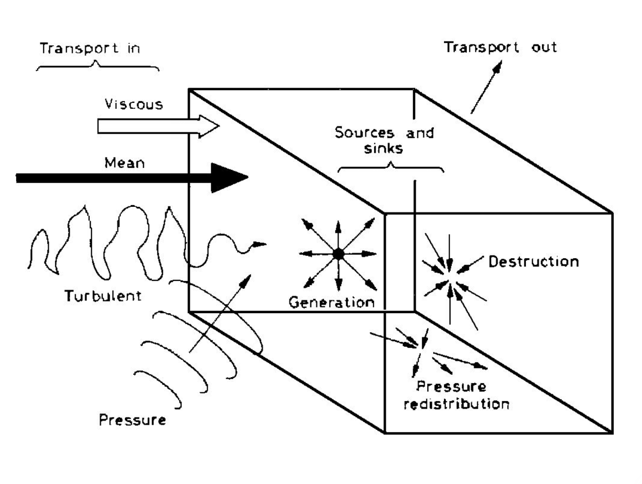
• <1>&<3>: the net rate of transport of \(\frac{1}{2}q^2\)

  <1>: the advection, mean energy transport, the rate of change of \(\frac{1}{2}q^2\) along a mean streamline

  <3>: turbulence transport

• <2>: pressure diffusion, net loss of turbulent energy by the work done in transporting the fluid through a region of changing pressure

  <2>&<3>: turbulent energy transport, energy diffusion

• <4>: an extraction of energy from the mean flow by the turbulence

  \(\frac{1}{2}q^2\) increases with a large shear on the flow

  energy production term, from the point of view of the turbulence

  energy loss term, from the point of view of the mean flow

  these same terms will appear in the mean flow kinetic energy equation with an opposite sign

  the only one involving a mean velocity gradient, the only term can act to take energy from the mean motion

  \(−ρ\overline{u'^2}\frac{∂U}{∂x}dxdydz\), the rate of work against the \(x\) component of the Reynolds normal stress to stretch an element of fluid \(dxdydz\) in the \(x\)-direction at a rate \(\partial U / \partial x\)

  \(−ρ\overline{u'v'} \frac{\partial U} {\partial y} dxdydz\), more important, the rate of work against the shear stress \(−ρ\overline{u'v'}\) to shear an element of fluid at the rate \(∂U/∂y\)

Before term <5>, we need to derive the expression of turbulence dissipation \(\varepsilon\) from the mean flow viscous term

• \(\left(\mu \frac{\partial U}{\partial y}\right) \frac{\partial U}{\partial y}\):

  the product of the instantaneous viscous stress and the instantaneous rate of strain,

  a transfer of energy between the bulk motion and the molecular motion,

  a dissipation of bulk kinetic energy into thermal energy by viscosity

  a source of energy, from the point of view of the temperature field, “aerodynamic” heating in high-speed flows

• the viscous term in the energy equation (the enthalpy equation) is: \[ \Phi=2 \mu S_{i j} \frac{\partial U_j}{\partial x_i}=\frac{\partial U_j}{\partial x_i}\left(\mu\left(\frac{\partial U_i}{\partial x_j}+\frac{\partial U_j}{\partial x_i}\right)\right)=\text { dissipation function } \]

  substitute the Reynolds decomposition and take the time average, we obtain \[ \bar{\Phi}=\frac{\partial \bar{U}_j}{\partial x_i}\left(\mu\left(\frac{\partial \bar{U}_i}{\partial x_j}+\frac{\partial \bar{U}_j}{\partial x_i}\right)\right)+\overline{\frac{\partial u'_j}{\partial x_i}\left(\mu\left(\frac{\partial u'_i}{\partial x_j}+\frac{\partial u'_j}{\partial x_i}\right)\right)} \]

  • 1^st term on \(RHS\) (\(=\Phi_m\)):

    dissipation of mean flow kinetic energy into thermal internal energy

    viscous diffusion of \(U\)

    the “direct” dissipation function

  • 2^nd term on \(RHS\) (=\(\varepsilon\)):

    viscous dissipation of turbulent kinetic energy

    the “turbulent”dissipation function

  We have \(\varepsilon >> \Phi_m\) since the instantaneous velocity gradients associated with the turbulence are much greater than the mean velocity gradients (except very close to a solid surface)

• <5> can be rewritten as: \[ \begin{aligned} &\nu\left(\overline{u' \nabla^2 u'}+\overline{v' \nabla^2 v'}+\overline{w' \nabla^2 w'}\right) \\ &=\nu\left(\frac{1}{2} \nabla^2\left(\overline{u'^2}+\overline{v'^2}+\overline{w'^2}\right)-\overline{\left(\frac{\partial u'}{\partial x}\right)^2}-\overline{\left(\frac{\partial u'}{\partial y}\right)^2}-\overline{\left(\frac{\partial u'}{\partial z}\right)^2}-\cdots\right) \\ \end{aligned} \] where the squares of velocity gradients as elements of \(\varepsilon\) (not all of them)

  the missing cross product terms (e.g. \(\mu\frac{\partial^2\overline{u'v'}}{\partial x\partial y}\)) are usually interpreted as a diffusion term, small, except near the wall

  \(\mu \frac{1}{2}\nabla^2\left(\overline{u'^2}+\overline{v'^2}+\overline{w'^2}\right) = \mu\nabla^2(\frac{1}{2}\overline{q^2})\), viscous diffusion of \(\frac{1}{2}q^2\)

  \(\mu\frac{\partial^2\overline{u'v'}}{\partial x\partial y}\), viscous diffusion of \(\overline{u'v'}\), small at all Reynolds numbers that are not too low as \[ \mu \overline{\left(\frac{\partial u_j}{\partial x_i}\right)^2} \approx \varepsilon \approx \mu\left(\overline{u^{\prime} \nabla^2 u^{\prime}}+\overline{v^{\prime} \nabla^2 v^{\prime}}+\overline{w^{\prime} \nabla^2 w^{\prime}}\right) \] And <5> can be finally written as: \[ \nu \overline{u_i\frac{\partial^2 u_i}{\partial x_j^2}} = \nu \frac{\partial^2\left(\frac{1}{2}q^2\right)}{\partial x^2_j} - \nu \overline{\left(\frac{\partial u_i}{\partial x_j}\right)^2} \]

Note this equation does NOT close the model still, the 3^rd order term <3> still exist, because this equation is based on the Reynolds Stress equation derived in the last section.

One way is the eddy viscosity models and the boussinesq assumption^[7] with which the turbulence fluctuation can be modelled (with an effective turbulence viscosity times mean flow velocity gradients), and the model is closed, with extra varies turbulence models.

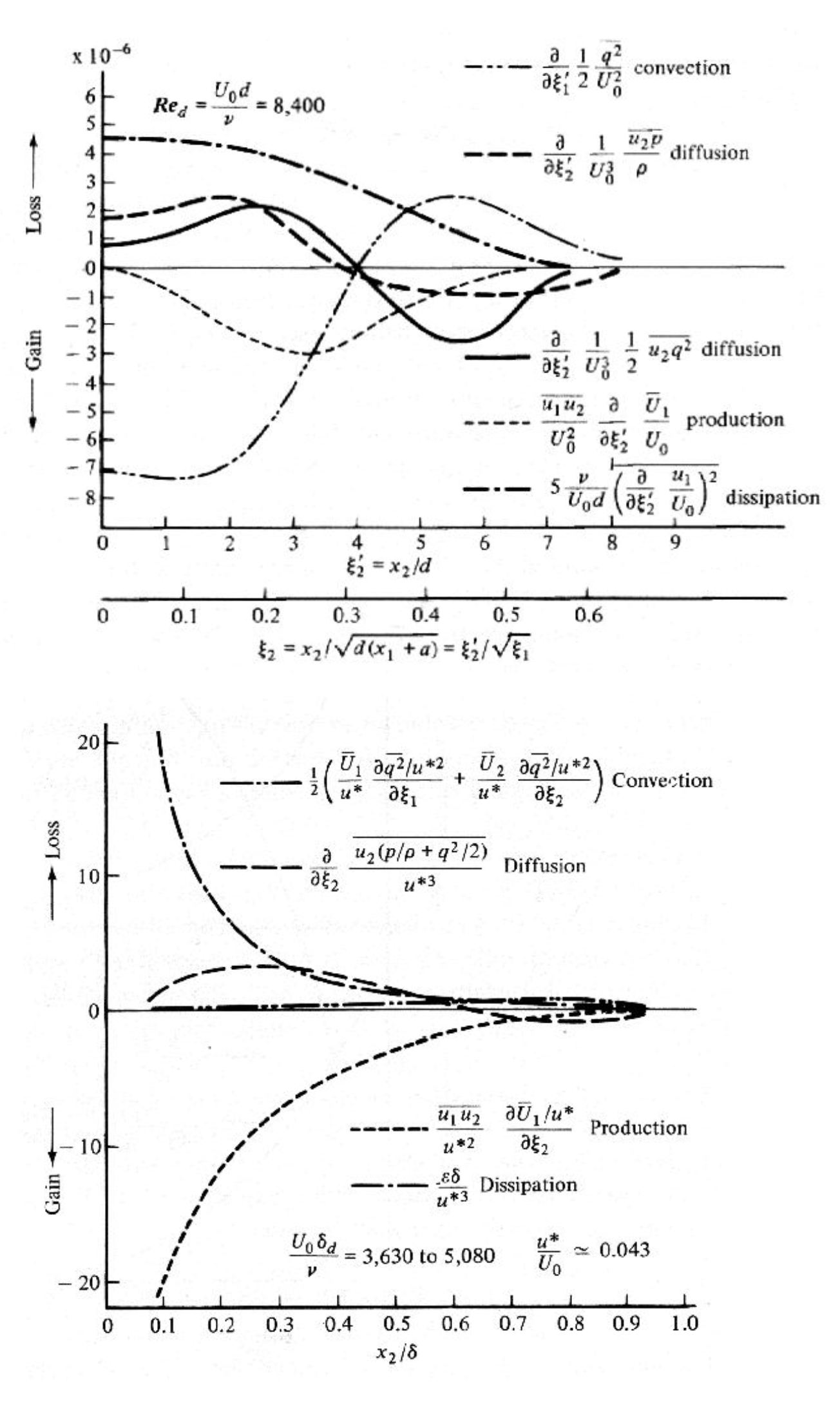
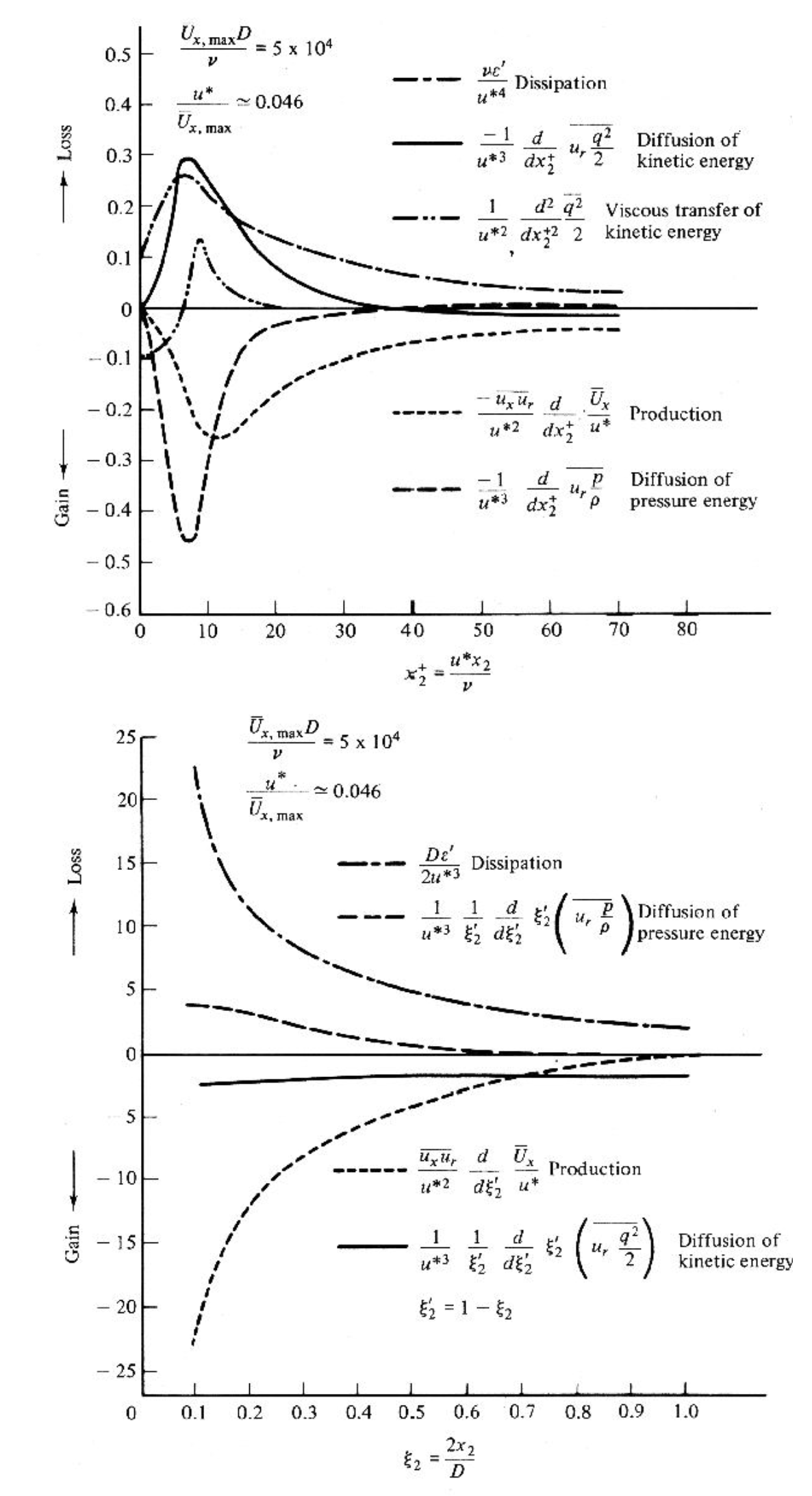
Energy balances (turbulence kinetic energy budget) diagram for the wake of a circular cylinder, zero pressure gradient boundary layer (outer scaling), a fully developed pipe flow (wall region (inner scaling) and core region (outer scaling)) is compared below:

• The wall bounded flows (boundary layer and pipe)
  • production term is approximately balanced by the dissipation term in large regions
  • diffusion terms become important
    • near the wall
    • near the outer edge of the layer, since all other terms become very small there
• The wake flow is somewhat more complicated
  • all terms appear to be important everywhere

Similar diagrams are shown below, results of jet flow, and DCBL of atmosphere

Note in atmosphere science, the buoyancy term is not negligible in N-S equation as well as the TKE equation,

\[\delta_{i 3} \frac{g}{\bar{\theta}_v}\left(\overline{u_i{ }^{\prime}{\theta}_v{ }^{\prime}}\right)\]

buoyant production or consumption term, a production or loss depending on whether the heat flux \(\overline{u_i{ }^{\prime}{\theta}_v{ }^{\prime}}\) is positive (during daytime over land) or negative (at night over land)

See more in turbulence kinetic energy - Climate Dynamics Group

Reference

1. Cantwell, B., & Coles, D. (1983). An experimental study of entrainment and transport in the turbulent near wake of a circular cylinder. Journal of fluid mechanics, 136, 321-374. ↩︎
2. Perry, A. E., & Tan, D. K. M. (1984). Simple three-dimensional vortex motions in coflowing jets and wakes. Journal of Fluid Mechanics, 141, 197-231. ↩︎
3. Blackwelder, R. F., & Kaplan, R. E. (1976). On the wall structure of the turbulent boundary layer. Journal of Fluid Mechanics, 76(1), 89-112. ↩︎
4. Spina, E. F., Donovan, J. F., & Smits, A. J. (1991). On the structure of high-Reynolds-number supersonic turbulent boundary layers. Journal of Fluid Mechanics, 222, 293-327. ↩︎
5. Robinson, P. A. (1997). Nonlinear wave collapse and strong turbulence. Reviews of modern physics, 69(2), 507. ↩︎
6. Townsend, A. A. R. (1980). The structure of turbulent shear flow. Cambridge university press. ↩︎
7. Boussinesq, J. (1877). Essai sur la théorie des eaux courantes. Impr. nationale. ↩︎
8. Bogey, C., & Bailly, C. (2006). Computation of the self-similarity region of a turbulent round jet using large-eddy simulation. In Direct and Large-Eddy Simulation VI (pp. 285-292). Springer, Dordrecht. ↩︎