hand written SPH method

under construction...

After inspecting the CUDA Particles simulation template. A simplest SPH model is implemented based on it.

Introduction

Related works

The first open-source SPH library ever is SPHysics FORTRAN code. It is developed by researchers at the Johns Hopkins University (US), the University of Vigo (Spain), the University of Manchester (UK), and the University of Rome, La Sapienza.

The earliest CUDA-based SPH is GPUSPH, (GitHub gpusph)^[1]. It is based on the CUDA Particles simulation template^[2], the same code reviewed in the last blog. And the newest release is version 5.0.

Besides, DualSPHysics, (GitHub DualSPHysics)^[3], a directly inherited variation from the SPHysics. Provides similar implementations with several optimization strategies. It is called "dual" because it supports both CPU and GPU implementations of the core functions.

Resources: SPH-Tutorial^[21] by SPlisHSPlasH, SPH Learning Notes

Simplifications

Compared with the matured developed SPH code, see DualSPHysics User Guide^[13], lots of simplifications are made in order to implement a simplest version of SPH code.

Verlet Scheme

There are two methods for numerical integration schemes, Verlet^[6] and mainstream Symplectic^[7] applied in DualSPHysics. The first is computationally simple with low stability. The second is a two-step prediction-correction method with higher stability. I choose the 1st order Euler backward and Verlet for simplification.

Kernel function

The performance of an SPH model depends heavily on the choice of the smoothing kernel. Instead of the Cubic Spline kernel ^[9] and Quintic Wendland kernel^[10], the Poly6, Spicky and Viscosity kernel functions are applied followed work of Müller et. al^[15].

Formulations List

These are the formulation list:

• Neighbor list
  • Domínguez^[19]
• Time integration scheme:
  • Euler backward
  • Verlet^[6]
  • Symplectic^[7]
• Variable time step
• Kernel functions:
  • Cubic Spline kernel ^[9]
  • Quintic Wendland kernel ^[11]
  • Poly6, Spicky and Viscosity kernel^[15]
• Pressure formulation (WCSPH)
  • Ideal gas equation^[16]
  • Monaghan/Tait equation^[12]
  • Pressure Poisson equation^[17]
• Viscosity formulation:
  • Artificial viscosity ^[4]
  • Laminar viscosity^[22]
  • Laminar viscosity^[22] + SPS turbulence model^[23][5]
• Density treatment:
  • Delta-SPH formulation ^[10]
• Boundary condition
  • Dynamic particles^[18]
  • Virtual particles^[12]
  • Mirroring particles^[20]

Update Step by Step

The fundamental algorithm is very similar to the CUDA demo^[2], only needs several changes for the control functions.

Stage 1: Neighboring searching

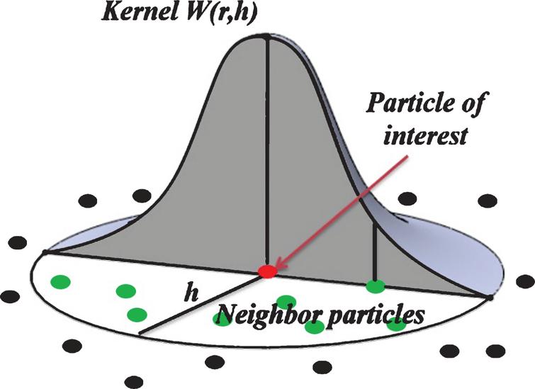
Theorem: Influence area

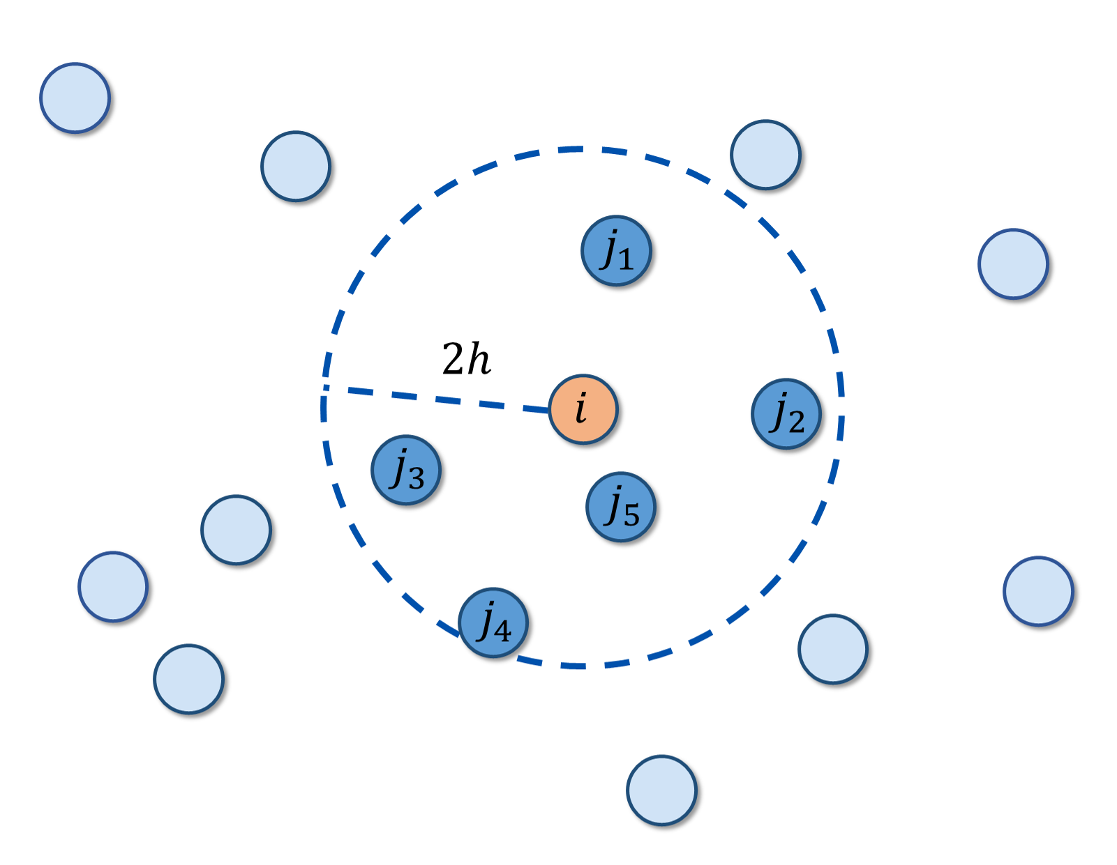
The influence area illustration of SPH is shown above. The circles denoted by \(i\), \(j\) represent the target particle and the interacting particles, respectively. The target particle only interacts with particles within the circle (dashed) with a radius of \(dist_{critic} = 2h\). With \(q = {dist}/{h}\) denoting the non-dimensional distance between two particles. \(q_{critc} = 2\) is the non-dimensional influence radius of the target particle.

The original \(dist_{critc}\) in the demo^[2] is the sum of the radius of the two interacting particles, i.e. \(dist_{critc} = 2 radius\) in the case of uniform radius particles. And \(h_{critic} = radius, q_{critic} = 1\).

There are two ways of defining \(h\),

By \(coefh\) (default 1): \[ h = coefh \cdot \sqrt{dx^2+dy^2+dz^2} \cdot dp \]

\[ h = coefh \cdot \sqrt{dx^2+dy^2+dz^2} dp \] By \(hdp\) (default 1.5): \[ h = hdp \cdot dp \] where characteristic length \(dp\) is choice to be the original particle distance when generating them, \(dp = 2*radius\) in demo^[2].

There is no concept of "particle diameter" in SPH as in the collision model^[2].

In the case of particles with the same radius, for the collision model, the interaction boundary of the particles is the physical particle diameter. While in SPH, the interaction boundary is defined freely. Particles are only the discretized points in the space.

The length unit \(dp\) is just a physical length easy to choose.

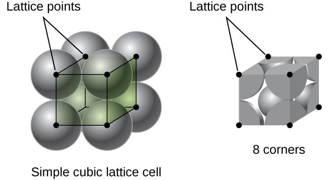
In the demo^[2], \(dp\) is equal to the diameter of particles. That means particles are generated (by function reset) tightly packed together, i.e. simple cubic stacking as shown below.

The second \(hdp\) method is applied in the code because of its simplicity. The equivalent \(hdp = 0.5\)

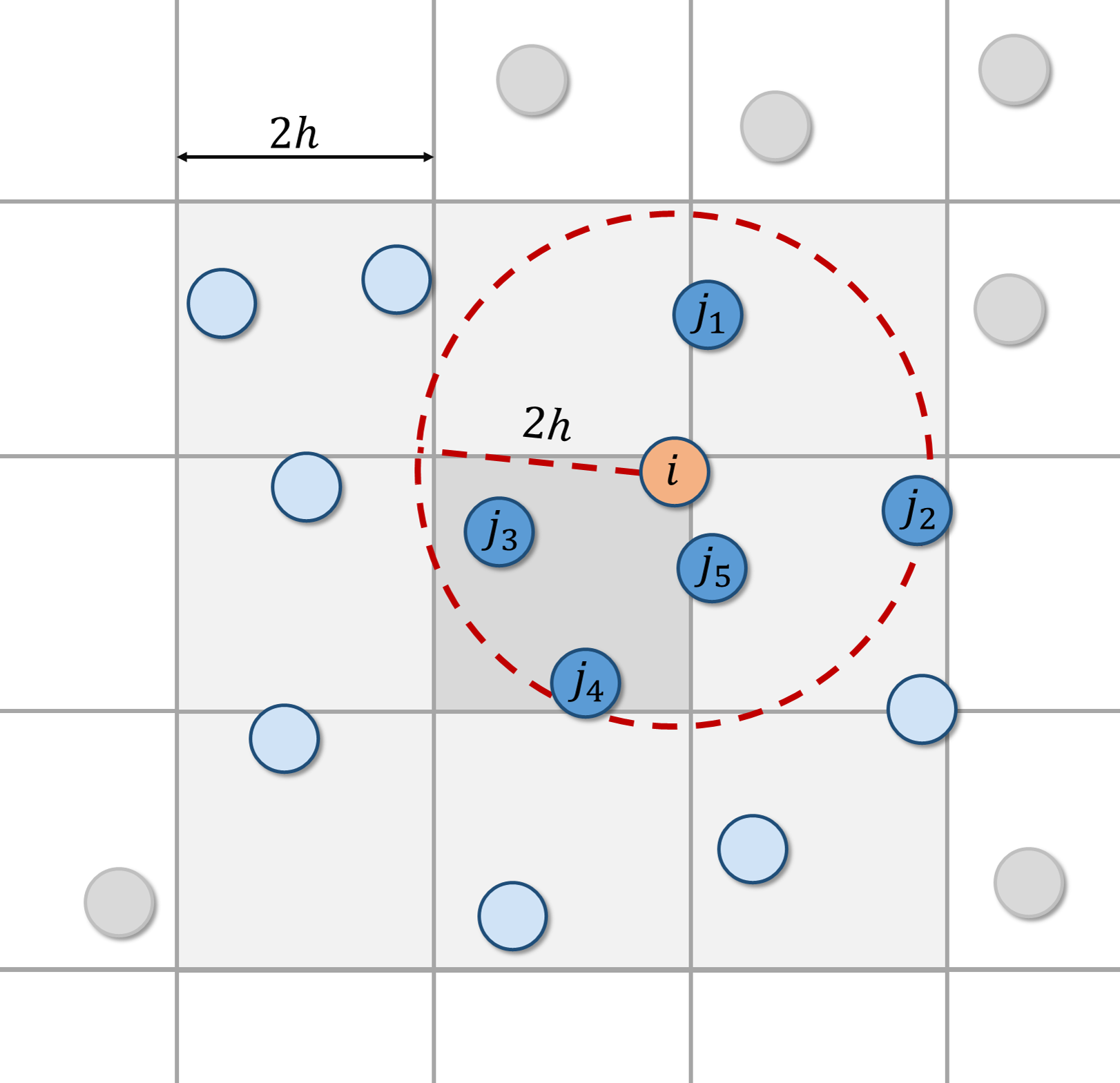
Algorithm: neighboring search

In order to find the true neighboring particles, instead of brute-force searching i.e. examining distances with all of the particles in the domain, a smart way is called neighboring search.

A grid as shown above is introduced, dividing the whole domain into cells. For each cell, a neighbor list containing all the particle ids in neighbor cells gets rebuilt periodically (every time step, or every 10-time step as in Hérault's work^[1]). When processing a target particle, the distances only get examined with particles in the neighbor list of its located target cell. In this way, the examining times are reduced dramatically and the shared memory can be well leveraged to avoid massive global memory access (not implemented here)

Grid span

At a glance, in the demo^[2], the grid is generated in the way that the grid spans \(dx, dy, dz\) equal \(dp\) as shown below in the code block.

float cellSize = m_params.particleRadius * 2.0f;  // cell size equal to particle diameter
m_params.cellSize = make_float3(cellSize, cellSize, cellSize);

Actually, the grid span is defined as the influencing distance \(2h\), as shown below. If the span is smaller, the interaction area will not be included by the neighboring area. Yet if the span is larger, the searching will not be the most efficient.

Note the term "grid" represents 3 different concepts:

• equal-space structured mesh, span \(2h\), divides the computational domain, e.g.

  "A grid is introduced, dividing the whole domain into cells"

  #define GRID_SIZE       64
  uint gridDim = GRID_SIZE;
  gridSize.x = gridSize.y = gridSize.z = gridDim;
  printf("grid: %d x %d x %d = %d cells\n", gridSize.x, gridSize.y, gridSize.z, gridSize.x*gridSize.y*gridSize.z);

• equal-space structured mesh, span \(dp\), used to generate a block of particles on its lattices, e.g.ParticleSystem::reset

  float jitter = m_params.particleRadius*0.01f;
  uint s = (int) ceilf(floor(powf((float) m_numParticles, 1.0f / 3.0f)*1000)/1000);
  uint gridSize[3];
  gridSize[0] = gridSize[1] = gridSize[2] = s;
  initGrid(gridSize, m_params.particleRadius*2.0f, jitter, m_numParticles);

• The GPU grid containing blocks of blockSize when running on the device e.g. in the code:

  // compute grid and thread block size for a given number of elements
  void computeGridSize(uint n, uint blockSize, uint &numBlocks, uint &numThreads)
  {
      numThreads = min(blockSize, n);
      numBlocks = iDivUp(n, numThreads);
  }
  
  void collide()
  {
      // thread per particle
      uint numThreads, numBlocks;
      computeGridSize(numParticles, 64, numBlocks, numThreads);
  
      // execute the kernel
      collideD<<< numBlocks, numThreads >>>();
  }

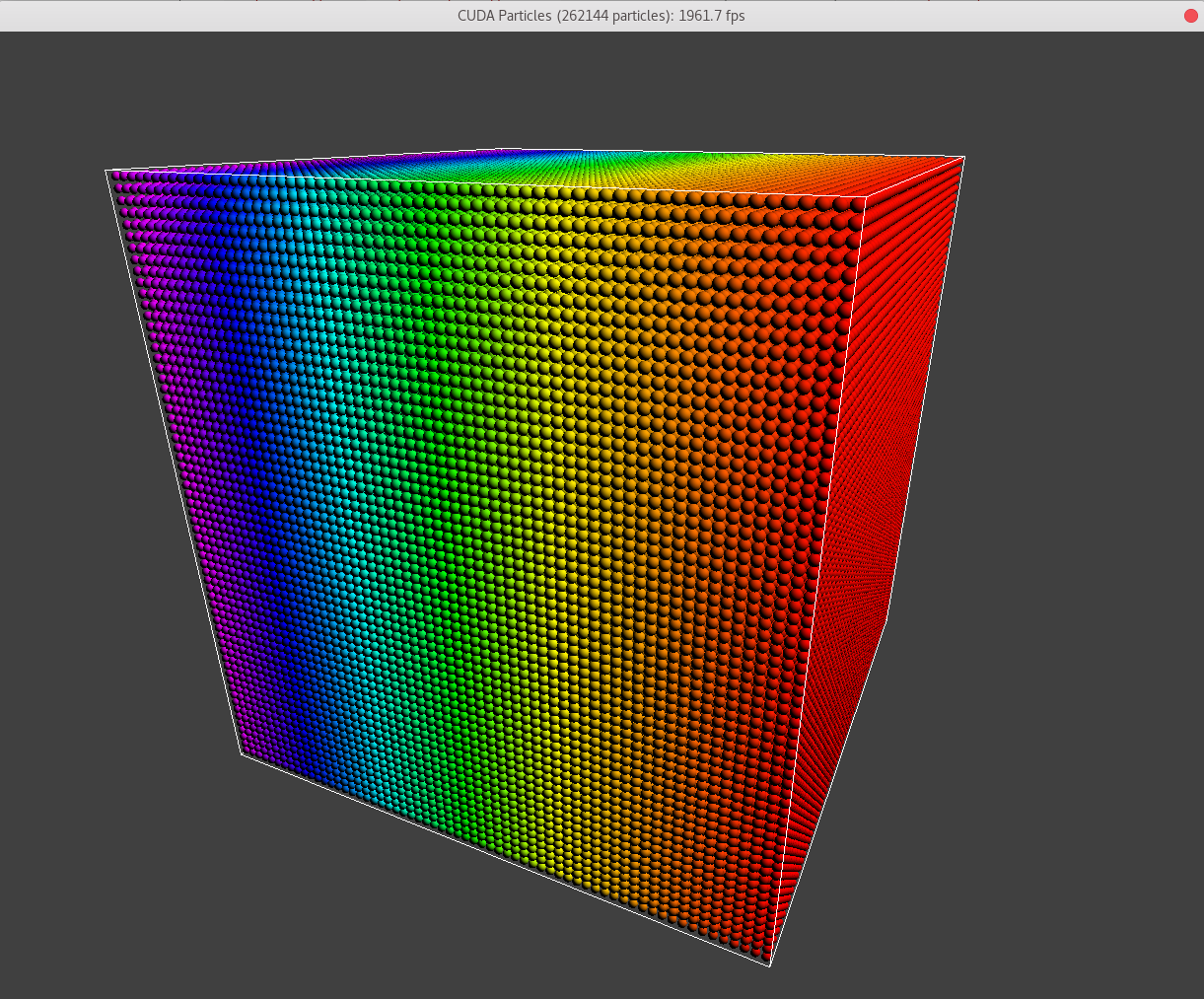
In demo^[2], when particle numbers are \(64\times64\times64 = 262144\), the first two grids coincide with each other. And \(262144\) is the maximum particle number according to the domain. And numBlocks = 4096.

Wait, there is another tiny difference (It turns out that we are lucky to be able to leave it but it is important to know this).

There are two ways of Building the Grid. One simple approach is via Atomic Operations, which is well illustrated by demo^[2]. In this approach, we allocate two arrays to the global memory:

• gridCounters – this stores the number of particles in each cell so far. It is initialized to zero at the start of each frame.
• gridCells – this stores the particle indices for each cell, and has room for a fixed maximum number of particles per cell.

Why fixed maximum number of particles per cell? It is because it is inefficient (nearly impossible) for GPU to allocate memories dynamically, which means the maximum number of particles per grid cell must be pre-defined.

In the scenario of demo^[2], this maximum number is easy to choose as the distance between particles is limited. Because particles in the collision model are rigid bodies and overlapping is not allowed, the maximum is set to be 4 particles per grid cell in the demo^[2], taking the assumption of simple cubic stacking. But in SPH, there is no such limitation as discussed above. We must make careful assumptions about it when we use the Atomic Operations method to build the grid.

Luckily, we are using the second approach, via sorting, slightly difficult to understand, also well illustrated in the demo^[2], and no need for the limitation of the maximum particles per cell.

Yet in Hérault's work^[1], the maximum lenth of the neighboring list is pre-defined, so that the examining loop is further unrolled during compilation for efficiency. We are not going to do that at the first time although is it easy to apply.

code

original

The distance examination is applied in __device__ float3 collideSpheres as:

__device__
float3 collideSpheres(float3 posA, float3 posB,
                      float3 velA, float3 velB,
                      float radiusA, float radiusB,
                      float attraction)
{
    // calculate relative position
    float3 relPos = posB - posA;

    float dist = length(relPos);
    float collideDist = radiusA + radiusB;

    float3 force = make_float3(0.0f);

    if (dist < collideDist)
    {
        // force += ...
    }

    return force;
}

The radius of two particles are set to be different, not suitable for SPH model.

update

step 0: house keeping

• comment out collider for simplicity and any function related to it such as: M_MOVE mode and its controller.

step 1: parameters/arguments, functions renaming, switching and introducing

• Rename the functions and params from collision related to SPH related such as:

  collideSpheres() -> SPHParticles()
  collideDist -> interactDist

• Introduce dp into params (i.e. struct SimParams), change grid span for generating the particles from particle diameter to dp, change the domain grid span to 2*h

• Introduce hdp,h into params, set hdp=0.5 and h=hdp*dp

• Make dp and hdp modifiable by flag via getCmdLineArgumentFloat

step 2: In function SPHParticles, change the distance limitation interactDist to 2*h so that distance limitation same as before.

• The original __device__ float3 collideSpheres is changed to be:

  __device__
  float3 SPHParticles(float3 posA, float3 posB,
                        float3 velA, float3 velB,
                        float h, float attraction)
  {
      // calculate relative position
      float3 relPos = posB - posA;
  
      float dist = length(relPos);
      float interactDist = 2*h;
  
      float3 force = make_float3(0.0f);
  
      if (dist < interactDist)
      {
          // force += ...
      }
  
      return force;
  }

• minor cleanups

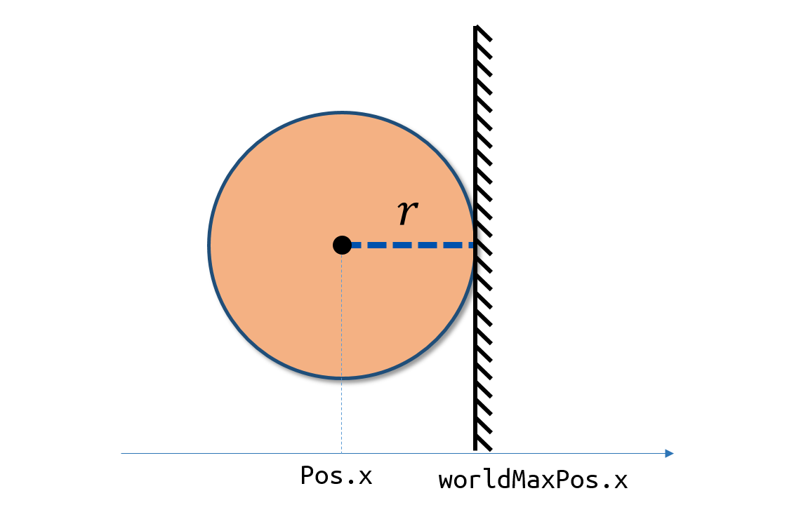
  • The boundary condition is parameterized for different setting of gridsize other than 64. A new parameter worldMaxPos is introduced right after the worldOrigin parameter as:

    if (pos.x > params.worldMaxPos.x - params.dp*0.5)
    {
        pos.x = params.worldMaxPos.x - params.dp*0.5;
        vel.x *= params.boundaryDamping;
    }

  • Add more flags operations such as gridLength

  • Another key factor introduced for dump all the parameters as:

    case 'k':
        psystem->dumpParameters();
        break;

Results of different hdps

./particles hdp=0.5	./particles hdp=0.8

Stage 2: Verlet time scheme

Theorem

Instead of the simple Euler backward time discretization scheme originally applied in the integration step, the Verlet scheme ^[6] is used such that: \[ \begin{aligned} \boldsymbol{v}_a^{n+1}&=\boldsymbol{v}_a^{n-1}+2 \Delta t \boldsymbol{F}_a^n \\ \boldsymbol{r}_a^{n+1}&=\boldsymbol{r}_a^n+\Delta t \boldsymbol{V}_a^n+0.5 \Delta t^2 \boldsymbol{F}_a^n \end{aligned} \]

For every \(N_s\) time steps: \[ \begin{aligned} \boldsymbol{v}_a^{n+1}&=\boldsymbol{v}_a^n+\Delta t \boldsymbol{F}_a^n \\ \boldsymbol{r}_a^{n+1}&=\boldsymbol{r}_a^n+\Delta t \boldsymbol{V}_a^n+0.5 \Delta t^2 \boldsymbol{F}_a^n \end{aligned} \]

Code

original

The DEM is implemented in two steps, i.e. two locations:

1. struct integrate_functor related params: gravity, globalDamping, boundaryDamping.
2. float3 SPHParticles() related params: spring, damping, shear.

The work flow in this stage is such that:

update

step 0: debug, the velocity update formula

• In original SPHD function, the new velocity is updated such that:

  newVel[originalIndex] = make_float4(vel + force, 0.0f);

  the velocity is added with the force without a multiplying of the delta time.

• Provide the SPHD with extra argument deltatime (changing SPH as well) and change the original code as:

  newVel[originalIndex] = make_float4(vel + deltaTime*force, 0.0f);

step 1: Rearrange integrate_functor and SPHD. Moving force out as a global parameter.

• In SPHD, the gravity (original in integrate_functor) and the collision forces (spring, damping, shear and attraction) are added to one argument force.
  • Delete the argument newVel in SPHD and SPH.
  • Add the argument newForce and update the force with gravity, the code structure as newVel:

  newForce[originalIndex]= make_float4(force, 0.0f);

• integrate_functor takes the argument force from SPHD and update the vel and pos as before (1st order Euler backword scheme).
  • Delete the force of globalDamping.

Note that In the original code, force is treated as temporal parameter, no memory of force needed.

step 2: rename the integrate_functor as integrate_verlet and update the vel and pos via the Verlet scheme

• integrate_verlet takes the pointer of step, vel_1 and vel_2 from outside, change these augments inside, mimicking the vel.
  • vel_1 and vel_2 indicates the velocity fields from last, and last of last step, respectively

step 3: debug, "nan" exists when updating the particles

• Inspect force, vel and pos of particles in dumpparticles

  found that the force returns "nan" because of the distance of two particles being 0.

• Add minimum distance condition to the updating force process in SPHParticles as:

  if (dist < interactDist && relPos.x > 1e-10 && relPos.y > 1e-10 && relPos.z > 1e-10 && relPos.x < -1e-10 && relPos.y < -1e-10 && relPos.z < -1e-10)

step 4: make deltaTime (0.04) and renderStep (10) as variables, changeable without recompilation. Print those information before rendering.

Result of Verlet time scheme

The nearly second order Verlet time scheme requires a much lower \(\Delta t\), for real time simulation, one-step-render-one-step-update is not applicable.

Stage 3: Control function

Theorem: SPH system

Instead of the DEM method that has been used for collision model, the control function between particles are changed, inspired by this notebook and work by Muller et. al^[15]

Density (Derived continuity equation):

\[ \rho(\boldsymbol{r_i}) = \sum_j m_j W_{poly6}(\boldsymbol{r_i} - \boldsymbol{r_j},h), \quad i\ne j \] where the the mass of all particles \(m =\rho_0\frac{4}{3}\pi*\left(\frac{dp}{2}\right)^3,dp=\frac{2}{64}.\) Weakly-compressible assumption is adopted, so the mass of each particle is fixed and the density varies.

Pressure (state equation):

Based on the state of equation by Desbrun^[16] \[ \begin{aligned} &P=k(\rho - \rho_0),\ \end{aligned} \]

where the rest density \(\rho_0=1000, k=3\).

Force (momentum equation):

Pressure force, gravity force and viscosity force is considered as: \[ \begin{aligned} \frac{d \boldsymbol{v_i}}{d t}&=-\sum_j\frac{1}{\rho_i}\nabla P_{j}+\boldsymbol{g}+\boldsymbol{\Gamma} \\ &= -\sum_j \left( m_j\frac{P_i+P_j}{2\rho_i\rho_j}\right)\nabla W_{spiky}(\boldsymbol{r_i} - \boldsymbol{r_j},h) + \boldsymbol{g}+\boldsymbol{\Gamma}, \quad i \ne j \\ \end{aligned} \] where the gravity force \(\boldsymbol{g} = (0, -1.0, 0) m/s^2\). \(\boldsymbol{\Gamma}\) is the dissipation terms, here, we only consider the linear viscosity^[22], i.e. \[ \begin{aligned} \boldsymbol{\Gamma}&=\mu\sum_jm_j\frac{\boldsymbol{v_j} - \boldsymbol{v_i}}{\rho_i \rho_j}\nabla^2 W_{viscosity}(\boldsymbol{r_i} - \boldsymbol{r_j},h),\quad i\ne j \end{aligned} \] where the viscosity of the fluid \(\mu = 5.0\)

Kernel function

\(W(\boldsymbol{r}, h)\) denotes the kernel function, we choose three different kernels. In 3D dimensions, they are defined as:

\[ \begin{aligned} &W_{poly6}(\boldsymbol{r}, h)=\frac{315}{64\pi h^9}\left(h^2-r^2\right)^3, \quad 0 \leq r \leq h \\ &W_{spiky}(\boldsymbol{r}, h)=\frac{15}{\pi h^6}\left(h-r\right)^3, \quad 0 \leq r \leq h \\ &\nabla W_{spiky}(\boldsymbol{r}, h)=-\frac{45}{\pi h^6}\left(h-r\right)^2\frac{\boldsymbol{r}}{r}, \quad 0 \leq r \leq h \\ &W_{viscosity}(\boldsymbol{r}, h)=\frac{15}{2\pi h^3}\left(-\frac{r^3}{2h^3}+\frac{r^2}{h^2}+\frac{h}{2r}-1\right), \quad 0 \leq r \leq h \\ &\nabla^2W_{viscosity}(\boldsymbol{r}, h)=\frac{45}{\pi h^6}\left(h-r\right), \quad 0 \leq r \leq h \\ \end{aligned} \]

Code

original

The collision force is calculated from the particle positions, plus some constants. Refer to the work flow in stage 2.

update

step 1: add more parameters

• define more vector parameters to particleSystem
  • float density
  • float pressure
• add more scalar parameters to particleSystem.params
  • mass, rho0, k

step 2: Add new file particles_kernel_functions.cuhto directory src, containing the Poly6, gradient of Spiky and Laplacian of Viscosity kernel functions

__device__
float poly6Kernel(float3 posA, float3 posB, float h)     //3-D
{ 
    float3 relPos = posB - posA;
    float dist = length(relPos);
    h = 2*h;
    float wker = 315.0f / 64.0f / PI / pow(h, 9) * pow(h*h-dist*dist,3); 
    return wker;
}

step 3: update density then pressure by function SPHDensityPressure

// accumulation density with another
__device__
float SPHDensityParticles(float3 posA, float3 posB,
                      float h, float mass)
{
    // calculate relative position
    float3 relPos = posB - posA;

    float dist = length(relPos);
    float interactDist = 2*h;

    float density = 0.0f;
    // float maxDist = params.dp /100.0f;

    if (dist < interactDist)
    {
        // density
        density = mass*poly6Kernel(posA, posB, h);
    }
    
    return density;
}

step 4: update force by function SPHForce, passing the resultant force to integrate_verlet

The final work flow in this stage is such that:

result

problem that still exist

boundary problem

To manifest better the problem, take a detail look at the numParticles = 80000 example,

angle 1	angle 2	angle 3

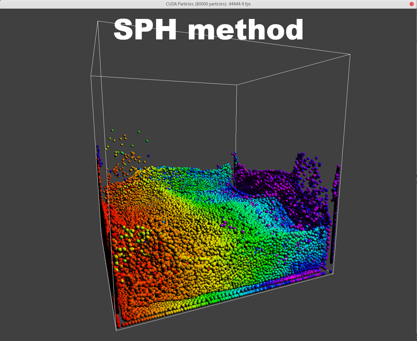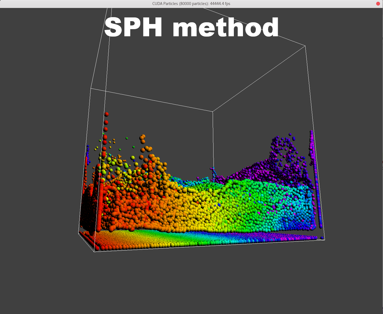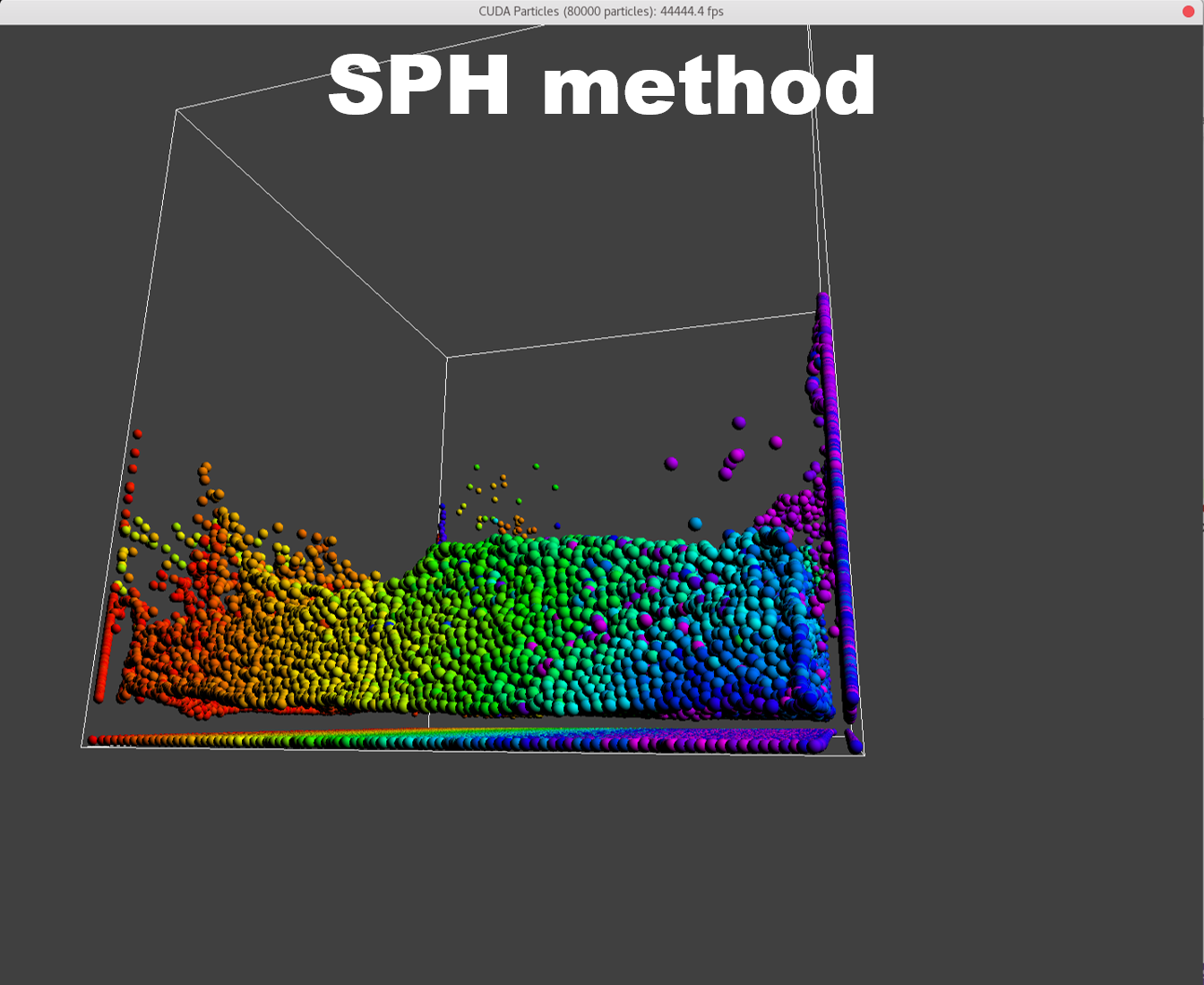A bunch of dense particles lay on the boundary resulting a huge density/pressure region, pushing the particles away from it, leaving a unphysical gap. Need a modification to the boundary.

Stage 4: Boundary

In former granular collision model^[2], the boundary condition can be provided precisely as the radius of the particle is physical.

To achieve the force of boundary to particles, following the work of Crespo at.al^[18], we arrange a layer of static particles regularly spanned on the boundary with same distance coefDp*dp. The density and pressure of the boundary particles is changed with the iteration, while the velocity and position of them remains the same.

code

update

Modify the arrangement of particles in initGrid. At first, arrange the bottom particles

for (uint z = 0; z < m_params.numNb + 1; z++)
{
    for (uint x = 0; x < m_params.numNb + 1; x++)
    {
        uint j = (z * (m_params.numNb + 1)) + x;
        m_hPos[j * 4] = (m_params.dp * m_params.coefDp * x) + m_params.worldOrigin.x;
        m_hPos[j * 4 + 1] = m_params.worldOrigin.y;
        m_hPos[j * 4 + 2] = (m_params.dp * m_params.coefDp * z) + m_params.worldOrigin.z;
        m_hPos[j * 4 + 3] = -1.0f;
    }
}

Then the other boundary particles arrange like this.

To improve the efficiency on boundary top, we don't arrange particles there and the we arrange particles on surrounding faces with a certain height coefBh * (woldMaxPos.y - worldOriginPos.y) .

result

After validation, the particle system works better when the distance of boundary particles is 0.6dp. Choose coefBh as 2/3.

Stage 5: Multiple GPU

Problems

The CUDA environment does not support, natively, a cooperative multi-GPU model. The model is based more on a single-core, single-GPU relationship. This works really well for tasks that are independent of one another, but is rather a pain if you wish to write a task that needs to have the GPUs cooperate in some way.

Algorithm, compared with multi-GPU machine learning, Halo Exchange might be needed: Parallel Paradigms and Parallel Algorithms – Introduction to Parallel Programming with MPI

• GPU peer-to-peer communication model provided as of the 4.0 SDK version or CPU-level primitives to cooperate at the CPU level
• One-core or multi-core
• MPI or ZeroMQ

Calculate the theoretical speedup, and test for each roots.

Resources

Book CUDA Programming by Shane Cook

• Chapter 8 Multi-CPU and Multi-GPU Solutions

Book CUDA C Programming Guide by NVIDIA

• NOT Recommended

Course CUDA Multi GPU Training by NVIDIA

• NOT Free

Free course

• 06.streams and mutiple GPU

• 08.MPI-GPU cluster

• NOT Recommended

References

1. Hérault, A., Bilotta, G., & Dalrymple, R. A. (2010). Sph on gpu with cuda. Journal of Hydraulic Research, 48(sup1), 74-79. ↩︎
2. Green, S. (2008). CUDA Particles. Technical Report contained in the CUDA SDK, www.nvidia.com. ↩︎
3. Crespo, A. J., Domínguez, J. M., Rogers, B. D., Gómez-Gesteira, M., Longshaw, S., Canelas, R. J. F. B., ... & García-Feal, O. (2015). DualSPHysics: Open-source parallel CFD solver based on Smoothed Particle Hydrodynamics (SPH). Computer Physics Communications, 187, 204-216. ↩︎
4. Monaghan JJ. 1992. Smoothed particle hydrodynamics. Annual Review of Astronomy and Astrophysics, 30, 543- 574. ↩︎
5. Dalrymple RA and Rogers BD. 2006. Numerical modeling of water waves with the SPH method. Coastal Engineering, 53, 141–147. ↩︎
6. Verlet L. 1967. Computer experiments on classical fluids. I. Thermodynamical properties of Lennard-Jones molecules. Physical Review, 159, 98-103. ↩︎
7. Leimkuhler BJ, Reich S, Skeel RD. 1996. Integration Methods for Molecular dynamic IMA Volume in Mathematics and its application. Springer. ↩︎
8. Monaghan JJ and Kos A. 1999. Solitary waves on a Cretan beach. Journal of Waterway, Port, Coastal and Ocean Engineering, 125, 145-154. ↩︎
9. Monaghan JJ and Lattanzio JC. 1985. A refined method for astrophysical problems. Astron. Astrophys, 149, 135–143. ↩︎
10. Molteni, D and Colagrossi A. 2009. A simple procedure to improve the pressure evaluation in hydrodynamic context using the SPH, Computer Physics Communications, 180 (6), 861–872 ↩︎
11. Wendland H. 1995. Piecewiese polynomial, positive definite and compactly supported radial functions of minimal degree. Advances in Computational Mathematics 4, 389-396. ↩︎
12. Monaghan JJ. 1994. Simulating free surface flows with SPH. Journal of Computational Physics, 110, 399–406. ↩︎
13. Crespo, A. J. C., Dominguez, J. M., Gómez-Gesteira, M., Barreiro, A., & Rogers, B. (2011). User guide for DualSPHysics code. University of Vigo: Vigo, Spain. ↩︎
14. Qin, Y., Wu, J., Hu, Q., Ghista, D. N., & Wong, K. K. (2017). Computational evaluation of smoothed particle hydrodynamics for implementing blood flow modelling through CT reconstructed arteries. Journal of X-ray science and technology, 25(2), 213–232. https://doi.org/10.3233/XST-17255 ↩︎
15. Müller, M., Charypar, D., & Gross, M. (2003, July). Particle-based fluid simulation for interactive applications. In Proceedings of the 2003 ACM SIGGRAPH/Eurographics symposium on Computer animation (pp. 154-159) ↩︎
16. Desbrun, M., Gascuel, MP. (1996). Smoothed Particles: A new paradigm for animating highly deformable bodies. In: Boulic, R., Hégron, G. (eds) Computer Animation and Simulation ’96. Eurographics. Springer, Vienna. https://doi.org/10.1007/978-3-7091-7486-9_5 ↩︎
17. Koschier D, Bender J, Solenthaler B, et al. Smoothed Particle Hydrodynamics Techniques for the Physics Based Simulation of Fluids and Solids[J]. 2019. ↩︎
18. Crespo AJC, Gómez-Gesteira M and Dalrymple RA. 2007. Boundary conditions generated by dynamic particles in SPH methods. Computers, Materials & Continua, 5, 173-184 ↩︎
19. Domínguez, J. M., Crespo, A. J. C., Gómez‐Gesteira, M., & Marongiu, J. (2011). Neighbour lists in smoothed particle hydrodynamics. International Journal for Numerical Methods in Fluids, 67(12), 2026-2042. ↩︎
20. Libersky, L. D., Petschek, A. G., Carney, T. C., Hipp, J. R., & Allahdadi, F. A. (1993). High strain Lagrangian hydrodynamics: a three-dimensional SPH code for dynamic material response. Journal of computational physics, 109(1), 67-75. ↩︎
21. Koschier, D., Bender, J., Solenthaler, B., & Teschner, M. (2020). Smoothed particle hydrodynamics techniques for the physics based simulation of fluids and solids. arXiv preprint arXiv:2009.06944. ↩︎
22. Lo EYM and Shao S. 2002. Simulation of near-shore solitary wave mechanics by an incompressible SPH method. Applied Ocean Research, 24, 275-286. ↩︎
23. Gotoh H, Shao S, Memita T. 2001. SPH-LES model for numerical investigation of wave interaction with partially immersed breakwater. Coastal Engineering Journal, 46(1), 39–63. ↩︎