Solving Wave Equation in Different Languages

2D wave equation with Dirichlet boundary condition is solved in C++ (with blas and Lapack), Python (with numpy), Matlab and Julia. Euler backward in time and central finite difference in space discretisation methods are adopted.

The aim is to compare the scientific calculation related syntaxes between these 4 languages. And have simple a comparison on their performances.

Problem setup

Wave equation

Wave equation is used for describe the wave fields such as water waves, sound waves and electromagnetic waves. The equation is: \[ \mathbf{\ddot {U}}=C^2\mathbf{\nabla} ^{2}\mathbf{U} \] In 2D, the principle is: \[ \frac{\partial^2u}{\partial t^2} = C^2\left(\frac{\partial^2u}{\partial x^2}+\frac{\partial^2u}{\partial y^2}\right), \quad u = f(x,t) \] From the formula, we can see it is second order, linear, hyperbolic PDE. Although it can be solved analytically (by variable separation), but we ignore that fact and try to solved it numerically.

Initial condition

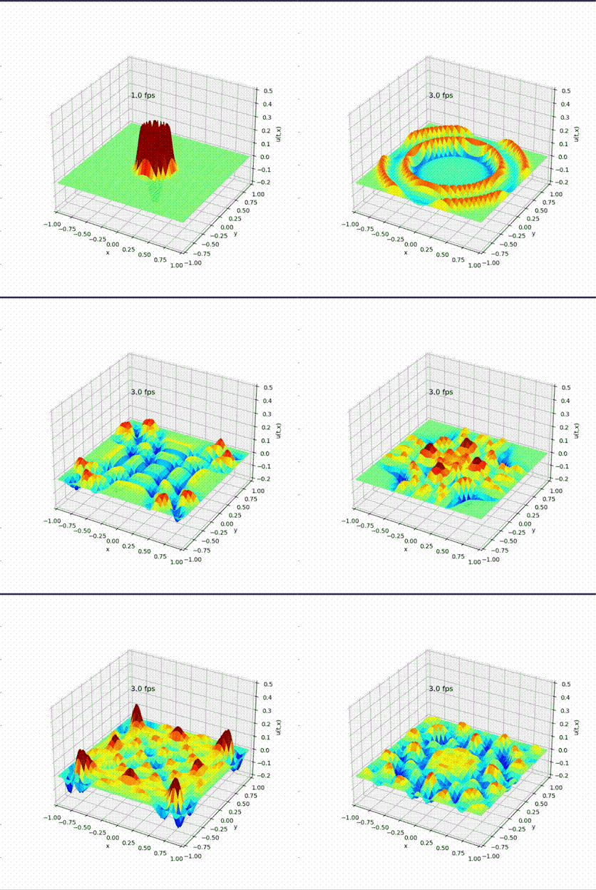
\[ u^0_{(x, y)}=\left[r_{(x, y)}^{4}-1\right]\left[\mathrm{e}^{-4 \omega^{2} r_{(x, y)}^{2}}-\mathrm{e}^{-4 \omega^{2}}-\frac{3}{4}\left(\mathrm{e}^{-\omega^{2} r_{(x, y)}^{2}}-\mathrm{e}^{-\omega^{2}}\right)\right] . \]

Boundary condition

Dirchlet boundary is adopted, i.e. all the \(u\) at the boundary is a fixed value 0;

Finite difference methods

Time Derivative Discretisation

Central difference is adopted, with a equal space time-step \(dt\): \[ \begin{aligned} \left[\frac{\partial^2u}{\partial t^2}\right]^k_{ij} =& \frac{v^{k}_{ij}-v^{k-1}_{ij}}{dt}, \\ \text{where} \quad v^k_{ij} = \left[\frac{\partial u}{\partial t}\right]^k_{ij} =& \frac{u^{k+1}_{ij}-u^{k}_{ij}}{dt} \end{aligned} \]

Space Derivatives Discretisation

Central difference is adopted, with a equal-space orthogonal cartesian mesh (\(dx\) for horizontal and \(dy\) for vertical), the derivatives become: \[ \begin{aligned} \left[\frac{\partial^2u}{\partial x^2}\right]^k_{ij} = \frac{u^k_{i+1,j}-2u^k_{ij}+u^k_{i-1,j}}{dx^2} \\ \left[\frac{\partial^2u}{\partial y^2}\right]^k_{ij} = \frac{u^k_{i,j+1}-2u^k_{ij}+u^k_{i,j-1}}{dy^2} \end{aligned} \]

Desirable result
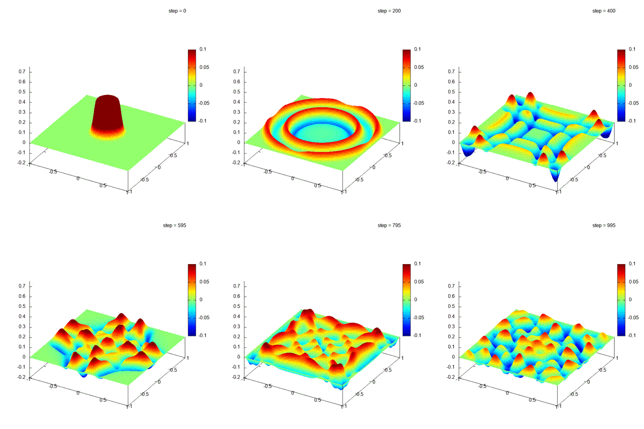
Desirable result

Iteration steps

Element-wise loop:

This method is adopted in the Codes section. It is efficient for this problem, but the scalability is poor and not used in reality.

  1. \[ u^{k+1}_{ij} = u^k_{ij}+v^k_{ij}dt \]

  2. \[ v^{k+1}_{ij} = Cdt\left(\frac{u^{k+1}_{i+1,j}-2u^{k+1}_{ij}+u^{k+1}_{i-1,j}}{dx^2} + \frac{u^{k+1}_{i,j+1}-2u^{k+1}_{ij}+u^{k+1}_{i,j-1}}{dy^2}\right) + v^{k}_{ij} \]

Matrix operation form:
  1. \[ \mathbf{U^{k+1}} = \mathbf{V^{k}} dt + \mathbf{U^{k}} \]

  2. In most of the cases, the 2D matrix is flattened into an 1D column vector*, and the formula turns into: \[ \mathbf{V}^{k+1} = C^2dt\mathbf{AU}^{k+1}+\mathbf{V}^{k} \] where \[ \mathbf{A}=\left[\begin{array}{cccccccc} e & a & & b & & & &&& \\ a & e & a & & b & & &&& \\ & \ddots &\ddots & \ddots& & \ddots & &&\\ b & & a & e & a & & b&&&\\ & \ddots& & \ddots & \ddots & \ddots & &\ddots&& \\ & & b & & a & e & a & &b& \\ & & & \ddots & & \ddots& \ddots & \ddots& &\\ & & & & b & & a& e & a& \\ & & & & & b & & a& e & \end{array}\right], \quad \mathbf{U} = \left[\begin{array}{c} u_{00} \\ u_{10} \\ \vdots \\ u_{01} \\ u_{21} \\ \vdots \\ \vdots \\ \vdots \\ u_{mn} \end{array}\right], \quad \mathbf{V} = \left[\begin{array}{c} v_{00} \\ v_{10} \\ \vdots \\ v_{01} \\ v_{21} \\ \vdots \\ \vdots \\ \vdots \\ v_{mn} \end{array}\right] \]

    \[ \text{which }\quad a = \frac{1}{dx^2}, \qquad b = \frac{1}{dy^2}, \qquad e = -\frac{2}{dx^2}-\frac{2}{dy^2} \]

  3. Set the boundary values back to 0

*If the matrix is not flattened:

In 2D case, the equivalent matrix operations formula is: \[\mathbf{V^{k+1}} = \left(\frac{C^2dt}{dx^2}\mathbf{U^{k+1}}\begin{bmatrix}1 & 1 & & & & \\ & -2 & 1 & & & \\ & 1 & -2 & \ddots & & \\ & & 1 & \ddots & 1 & \\ & & & \ddots & -2 & \\ & & & & 1 & 1 \\\end{bmatrix}+\frac{C^2dt}{dy^2}\begin{bmatrix}1 & & & & & \\1 & -2 & 1 & & & \\ & 1 & -2 & 1 & & \\ & & \ddots & \ddots & \ddots & \\ & & & 1 & -2 & 1 \\ & & & & & 1 \\\end{bmatrix} \mathbf{U^{k+1}}\right) + \mathbf{V^k}\] Unfortunately this formula isn't provided in all the mature CFD codes. Maybe because it requests 2 matrix MULTI-ADDs at one step, but the main reason is that when dealing with unstructured mesh i.e. nodes are located freely in the space, not on a cartesian grid, the 2D matrix cannot be used.

*The matrix is flattened in column major way, for example: \[\left[\begin{array}{lll}u_{00} & u_{01} & u_{02} \\u_{10} & u_{11} & u_{12} \\u_{20} & u_{21} & u_{22}\end{array}\right] \Rightarrow\left[\begin{array}{c}u_{00} \\u_{10} \\u_{20} \\u_{01} \\\vdots \\u_{22}\end{array}\right]\]

Codes

All the codes are available here: solve-wave-equation. Central difference in time and space, element-wise operations are applied.

Python, Julia, Matlab

These 3 languages have very similar syntaxes, as shown below:

Scroll horizontally to see all the codes.

Python Julia Matlab
import matplotlib.pyplot as plt
import numpy as np
import time

# define parameters
nSteps = 1000  		# Number of timesteps
Dt = 1e-3  				# Length of a timestep
C = 15  					# Stiffness constant, sqaure of wave speed
nx = 300  				# Number of x support points
ny = 300  				# Number of y support points
w = 20  					# Initial wave width

# Domain size (-xmax<x<xmax, -ymax<y<ymax)
xmax = 1
ymax = 1

# Initialise the arrays with initial values.
Dx = 2 * xmax / nx
Dy = 2 * ymax / ny
[y, x] = np.meshgrid(np.arange(-ymax, ymax + Dy, Dy), np.arange(-xmax, xmax + Dx, Dx))
r = np.square(x) + np.square(y)
v = np.zeros(np.shape(x))
u = np.zeros(np.shape(x))
pos = (r < 1)
u[pos] = np.exp(-4 * w**2 * np.square(r[pos])) - 0.75 * np.exp(-w**2 * np.square(r[pos]))
u[pos] = u[pos] + 0.75 * np.exp(-w**2) - np.exp(-4 * w**2)
u[pos] = u[pos] * (np.power(r[pos], 4) - 1)

# Loop over timesteps
plt.ion()
fig, ax = plt.subplots(figsize=(7, 7), subplot_kw={"projection": "3d"})
fig.canvas.draw()

tic = time.perf_counter()
for step in range(nSteps):
    u[1:-1, 1:-1] = u[1:-1, 1:-1] + Dt * v[1:-1, 1:-1]
    v[1:-1,1:-1]  = v[1:-1,1:-1]+ \
                (C*Dt/(Dx**2))*( u[0:-2,1:-1] - 2.*u[1:-1,1:-1] + u[2:,1:-1] )+ \
                (C*Dt/(Dy**2))*( u[1:-1,0:-2] - 2.*u[1:-1,1:-1] + u[1:-1,2:] )

    if step % 5 == 0:
        ax.clear()
        ax.plot_surface(x, y, u, cmap=plt.cm.winter,vmin=-0.1, vmax=0.1)
        toc = time.perf_counter()
        ax.text(-1, 1, 0.2, str(np.floor(1/(toc-tic)))+" fps",fontsize=12)
        tic = time.perf_counter()
        ax.set_xlim([-1, 1])
        ax.set_ylim([-1, 1])
        ax.set_zlim([-0.2, 0.5])
        ax.set_xlabel('x')
        ax.set_ylabel('y')
        ax.set_zlabel('u(t,x)')
        plt.pause(0.001)
        fig.canvas.flush_events()
        
plt.ioff()

import PyPlot; # matplolib.PyPlot API is used for julia
const plt = PyPlot;
using Dates;

# define parameters
nSteps = 1000;          # Number of timeSteps
Dt = 1e-3;               # Length of a timeStep
C = 15;                  # Stiffness constant
nx = 300;                # Number of x support points
ny = 300;                # Number of y support points
w = 20;                  # Initial wave width

# Domain size (-xmax<x<xmax, -ymax<y<ymax)
xmax = 1;
ymax = 1;

# Initialise the arrays with initial values.
Dx = 2 * xmax / nx;
Dy = 2 * ymax / ny;
x = collect(-xmax:Dx:xmax) .* ones(ny + 1)'; # broadcasting is used to generate 2D array
y = collect(-ymax:Dy:ymax)' .* ones(nx + 1);
r = x .^ 2 + y .^ 2;
v = zeros(size(x));
u = zeros(size(x));
pos = r .< 1;
u[pos] = exp.(-4 * w^2 * r[pos] .^ 2) - 0.75 * exp.(-w^2 * r[pos] .^ 2);
u[pos] = u[pos] .+ 0.75 .* exp.(-w^2) .- exp.(-4 .* w^2);
u[pos] = u[pos] .* (r[pos] .^ 4 .- 1);

# Loop over timesteps
plt.ion();
fig, ax = plt.subplots(figsize=(7, 7), subplot_kw=Dict("projection" => "3d"));
fig.canvas.draw();

global tic = now();
for step in 0:nSteps
    u[2:nx, 2:ny] = u[2:nx, 2:ny] + Dt .* v[2:nx, 2:ny];
    v[2:nx, 2:ny] = v[2:nx, 2:ny] + 
                    (C * Dt / Dx^2) .* (u[1:nx-1, 2:ny] .- 2 .* u[2:nx, 2:ny] + u[3:nx+1, 2:ny]) + 
                    (C * Dt / Dy^2) .* (u[2:nx, 1:ny-1] .- 2 .* u[2:nx, 2:ny] + u[2:nx, 3:ny+1]);
    if step % 5 == 0
        ax.clear();
        ax.plot_surface(x, y, u, cmap=plt.cm.winter, vmin=-0.1, vmax=0.1);
        toc = now();
        ax.text(-1, 1, 0.2, string(floor(1000 / (toc - tic).value)) * " fps", fontsize=12);
        global tic = now();
        ax.set_xlim([-1, 1]);
        ax.set_ylim([-1, 1]);
        ax.set_zlim([-0.2, 0.5]);
        ax.set_xlabel("x");
        ax.set_ylabel("y");
        ax.set_zlabel("u(t,x)");
        plt.pause(0.001);
        fig.canvas.flush_events();
    end
end

plt.ioff();
% no package needed in matlab


% Define parameters
nSteps = 1000;            % Number of timesteps
Dt = 1e-3;                % Length of a timestep
C = 15;                   % Stiffness constant
nx = 200;                 % Number of support points in x
ny = 200;                 % Number of support points in y
w = 20;                   % Initial wave width

% Domain size (-xmax<x<xmax, -ymax<y<ymax)
xmax = 1;
ymax = 1;

# Initialise the arrays with initial values.
Dx = 2*xmax/nx;
Dy = 2*ymax/ny;
[y,x] = meshgrid(-ymax:Dy:ymax,-xmax:Dx:xmax);
r = x.^2 + y.^2;
v = zeros(size(x));
u = zeros(size(x));
pos = (r<1);
u(pos) = exp(-4*w^2*r(pos).^2) - 0.75*exp(-w^2*r(pos).^2);
u(pos) = u(pos) + 0.75*exp(-w^2) - exp(-4*w^2);
u(pos) = u(pos).*(r(pos).^4-1);

% Loop over timesteps
tic
for step = 0:nSteps
    u(2:nx,2:ny) = u(2:nx,2:ny) + Dt.*v(2:nx,2:ny);
    v(2:nx,2:ny) = v(2:nx,2:ny) ...
        +(C*Dt/Dx^2).*( u(1:nx-1,2:ny) - 2.*u(2:nx,2:ny) + u(3:nx+1,2:ny) ) ...
        +(C*Dt/Dy^2).*( u(2:nx,1:ny-1) - 2.*u(2:nx,2:ny) + u(2:nx,3:ny+1) );
    
    % Plot every 5 steps, otherwise too slow
    if (mod(step,5)==0)
        surf(x(1:5:end,1:5:end),y(1:5:end,1:5:end),u(1:5:end,1:5:end))
        colormap winter
        % shading interp
        % light
        axis equal;
        xlabel('x')
        ylabel('y')
        zlabel('u(t,x,y)')
        caxis([-.2, .2])
        axis([-xmax, xmax, -ymax ymax -0.2 0.5])
        hold on
        text(.8, 1, 0.2, strcat(num2str(floor(1/toc)), " fps"), 'FontSize', 12)
        tic
        hold off
        drawnow
    end
end


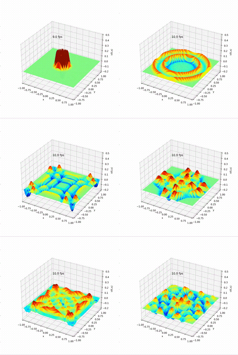
Python result

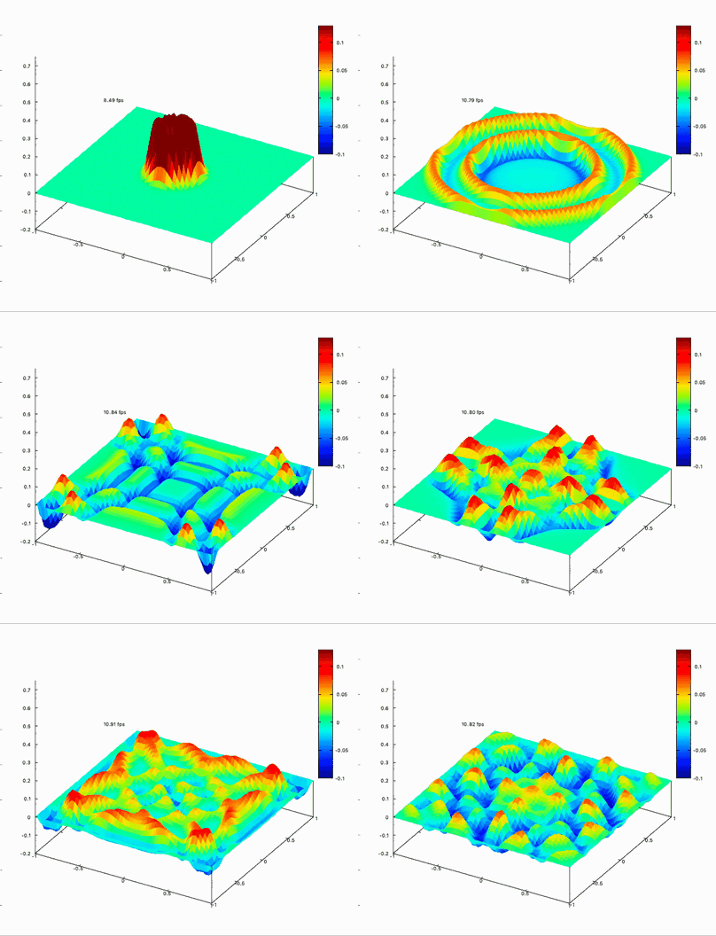
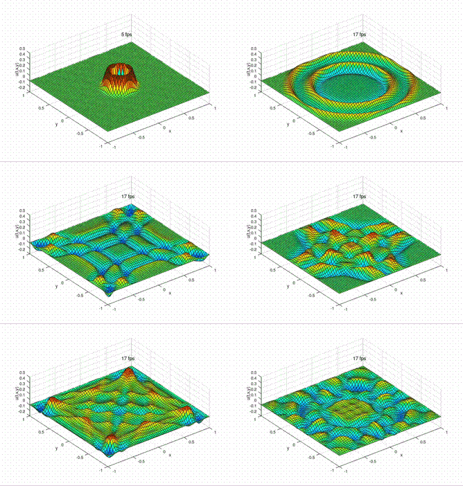
Julia result

Matlab result, implemented on Octave

C++

Because of the flexibility (difficulty) of C++, there are extra concerns as:

Matrix Datatype:

In order to take advantage of the efficiency of STL(standard template library) without worrying about the memory control, vector<double> is used to store the data to be calculated.

There are two ways of storing a 2D matrix,

  • 1D vector<double>, the most common way. The matrix is flattened as discussed above.
  • 2D vector<vector<double> >, consistent with the Python/Julia/Matlab codes.

How to represent a 2D matrix is not a c++ exclusive question. The languages above can also handling both 1D 2D matrix.

2D vector is adopted here for the sake of simplicity.

Matrix operations

There are 2 options for matrix operations

  • Nested 2-layer for-loops to conduct the element-wised operations. Serial and slow it seems to be, but thanks to the compiler, it will be optimised to be data-level-parallel and the speed is ok.

  • Besides, there is a fortran library BLAS (Basic Linear Algebra Subprograms), famous of the efficiency and high performance on matrix operations. BLAS has been widely used in the scientific computing field. It not only supports general full-populated matrix type, but also supports the triangular, symmetric and banded matrix computing. (Similar to the sparse matrix type in MATLAB, but less flexible)

Here I choose option 1, still working on option 2.

Since BLAS is written on Fortran, there are 2 ways of calling BLAS in C/C++

  • Calling the Fortran BLAS library in C++, need extra attention on the matrix storage method*, and the compiling method*
  • Use the CBLAS wrapper, may not work on all of the HPCs, but more convenient. The storage method can be pre-assigned when calling. No need to take care of the compiling method.

*With a 2D matrix, there are two ways of storage in the memory, row-major or column-major. The convention is row-major but on Fortran, it is column-major. \[\begin{aligned}Conventional:&\quad \left(\begin{array}{lll}a_{11} & a_{12} & a_{13} \\a_{21} & a_{22} & a_{23}\end{array}\right) \quad \text { stored as }[\underbrace{a_{11} a_{12} a_{13}}_{\text {Row } 1} \underbrace{a_{21} a_{22} a_{23}}_{\text {Row } 2}] \\Fortran:& \quad\left(\begin{array}{lll}a_{11} & a_{12} & a_{13} \\a_{21} & a_{22} & a_{23}\end{array}\right) \quad \text { stored as }[\underbrace{a_{11} a_{21}}_{\text {Col. } 1} \underbrace{a_{12} a_{22}}_{\text {Col. } 2} \underbrace{a_{13} a_{23}}_{\text {Col. } 3}]\end{aligned}\]

*The way Fortran and C++ compilers generate compiled forms of a function differ, so in order to use a Fortran code, we must tell the C++ compiler to look for the compiled symbol with a slightly different name than what it would otherwise expect. There are two main changes:

  • Fortran appends the function name with an underscore (_), whereas C/C++ compilers do not.

  • Since C++ supports function overloading (see Section 6.5), it “mangles” the function names with the parameter datatypes to ensure they are always unique.

In order to call Fortran 90 functions from our C++ code, we therefore need to add the underscore and turn off the name mangling.

Plotting methods:

Although there is no official plotting library in C++, there are many libraries available, such as: GNUPlot, Koolplot, MATLAB, matplotlib-cpp. See plotting package for c++ in detail. I prefer GNUPlot, a fast and powerful, widely used plotting library.

And There are two options of plotting,

  • Joint: Embedding GNUPlot with C++ (with gnuplot-iostream), updates the plot real-time with iteration.
  • Two-stage: First output all the data of every plotting step, then shade them with GNUPlot all together.

In order to keep align with the codes in the last section, I choose the Joint method here.

Main code

Some of the code is here:

Scroll horizontally to see the utils

main utils.hpp gnuplot-support.cpp
#define _USE_MATH_DEFINES
#include <iostream>
#include <vector> 
#include <cmath>
#include "utils.hpp"

using namespace std;

int main()
{
  // define parameters
  int nSteps = 1000;
  double Dt = 0.001;
  double C = 15;
  int nx = 300, ny = 300;
  double w = 20;

  // Domain size (-xmax<x<xmax, -ymax<y<ymax)
  double xmax = 1.0, ymax = 1.0;

  // Initialise the arrays with initial values.
  double Dx = 2 * xmax / nx;
  double Dy = 2 * ymax / ny;

	vector<double> x = linespace( -xmax,  xmax,  nx+1);
	vector<double> y = linespace( -ymax,  ymax,  ny+1);

	vector<vector<double> > X, Y, r, v, u;
	r.assign(y.size(), vector<double>(x.size()));
	v.assign(y.size(), vector<double>(x.size()));
	u.assign(y.size(), vector<double>(x.size()));

  meshgrid(x, y, X, Y);

	// initialization
	for (int j=0; j < ny+1; j++)
    {
    	for (int i=0; i < nx+1; i++)
        {
			r[j][i] = pow(X[j][i],2) + pow(Y[j][i],2);
			if(r[j][i]<1)
			{
				u[j][i] = exp(-4 * pow(w,2) * pow(r[j][i],2))\
                  - 0.75 * exp(-pow(w,2) * pow(r[j][i],2));
				u[j][i] = u[j][i] + 0.75 * exp(-pow(w,2)) - exp(-4 * pow(w,2));
				u[j][i] = u[j][i]*(pow(r[j][i], 4) - 1);
			}
        }
    }

	// Loop over timesteps
    GnuPlotWrapper<double> GPW;
	for (int step = 0; step < nSteps; step++)
	{
		for (int j=1; j < ny; j++)
		{
			for (int i=1; i < nx; i++)
			{
				u[j][i] = u[j][i] + Dt * v[j][i];
			}
		}

		for (int j=1; j < ny; j++)
		{
			for (int i=1; i < nx; i++)
			{
				v[j][i] = v[j][i] + 
				(C*Dt/(pow(Dx,2)))*(u[j][i-1]-2*u[j][i]+u[j][i+1])+ 
				(C*Dt/(pow(Dy,2)))*(u[j-1][i]-2*u[j][i]+u[j+1][i]);
			}
		}

        if (step%5 ==0)
        {
            GPW.update(x,y,u);
            usleep(1);
        }
	}
}


#include "gnuplot-support.cpp"

vector<double> linespace(double start, double ed, int num);
void meshgrid(vector<double> xin, vector<double> yin, 
              vector<vector<double>> &xout, 
              vector<vector<double>> &yout);
inline string time_diff(chrono::duration<double> elapsed_seconds);

template <class T>
class GnuPlotWrapper
{
public:
    GnuPlotWrapper()
    {
        init_style();
        start = chrono::system_clock::now();
    }

    inline void init_style()
    {
        gp << "set term qt size 700, 700 position 0,0\n";
        gp << "set xyplane at -0.2\n";
        gp << "set zrange [-0.2:0.75]\n";
        gp << "set cbrange [-0.1:0.13]\n";
        gp << "set hidden3d nooffset\n";
        gp << "set pm3d\n";
        // other unnecessary settings
    }

    void update(vector<T> &x, vector<T> &y, vector<vector<T>> &u, int step = 5)
    {
        pts_reset();
        for (auto i = 0; i < x.size(); i += step)
        {
            this->segment_reset();
            for (auto j = 0; j < y.size(); j += step)
            {
                this->seg_push_back(x[i], y[j], u[j][i]);
            }
            this->pts_push_back();
        }
        this->plot();
    }

private:
    inline void pts_reset()
    {
        pts.erase(pts.begin(), pts.end());
    }

    inline void segment_reset()
    {
        segment.erase(segment.begin(), segment.end());
    }

    inline void seg_push_back(T &x, T &y, T &z)
    {
        segment.push_back(MyTriple<T>(x, y, z));
    }

    inline void pts_push_back()
    {
        pts.push_back(segment);
    }

    inline void plot()
    {
        gp << "splot '-' w pm3d notitle\n";
        gp.send2d(pts);
        auto end = chrono::system_clock::now();
        gp << "set label 1 '" << time_diff(end - start) \
           << " fps' at -0.8,0,0.3\n";
        start = chrono::system_clock::now();
        gp.flush();
    }

private:
    Gnuplot gp;
    vector<vector<MyTriple<T>>> pts;
    vector<MyTriple<T>> segment;
    chrono::system_clock::time_point start;
};
#include <vector>
#include <cmath>
#include "gnuplot-iostream.h"

template <typename T>
struct MyTriple
{
    MyTriple() : x(0), y(0), z(0) {}
    MyTriple(T _x, T _y, T _z) : x(_x), y(_y), z(_z) {}

    T x, y, z;
};

// Tells gnuplot-iostream how to print objects of class MyTriple.
namespace gnuplotio
{
    template <typename T>
    struct BinfmtSender<MyTriple<T>>
    {
        static void send(std::ostream &stream)
        {
            BinfmtSender<T>::send(stream);
            BinfmtSender<T>::send(stream);
            BinfmtSender<T>::send(stream);
        }
    };

    template <typename T>
    struct BinarySender<MyTriple<T>>
    {
        static void send(std::ostream &stream, const MyTriple<T> &v)
        {
            BinarySender<T>::send(stream, v.x);
            BinarySender<T>::send(stream, v.y);
            BinarySender<T>::send(stream, v.z);
        }
    };

    template <typename T>
    struct TextSender<MyTriple<T>>
    {
        static void send(std::ostream &stream, const MyTriple<T> &v)
        {
            TextSender<T>::send(stream, v.x);
            stream << " ";
            TextSender<T>::send(stream, v.y);
            stream << " ";
            TextSender<T>::send(stream, v.z);
        }
    };
} // namespace gnuplotio

MyTriple<double> get_point(double &x, double &y, double &z)
{
    return MyTriple<double>(x, y, z);
}


Result

C++ realtime result

Benchmark on the matrix computing

The codes are evaluated without the I/O or rendering. With purely matrix computing, the time consumptions are:

Data is in result.md.

Compared with original code, Dt = 1e-5 to avoid the divergence when increasing the matrix dimension.

Conclusions

  • C++ is great!
    • Although 4 languages are covered, I feel like I spent my entire time writing C++. And the better performance over all the other interpreted codes makes me feel well paid off.
  • Python is great
    • Although Python is famous to be slow, but with numpy library (As far as I know, Anaconda numpy use OpenBLAS) it speed for matrix computation is not bad.
  • Julia is NOT fast, at my level
    • Actually, I wrote this blog aiming at learning Julia. I was hoping Julia can run as fast as C++ as they claimed. But the performance is the worst of all the codes. Maybe it is because of the JIM system. Or I need more time working on it.
    • Besides, the plotting is inefficient. Again, it is not quite fair because I used Julia to call python API. I haven't look into the plotting function in Julia.
    • For now, I'd rather use Python or MATLAB for quick preliminary developing and C++ for deploying.
  • MATLAB has a really efficient plotting method, even I use octave as a alternative for now. I wander if I can seek the same plotting performance on C++.
Solving Wave Equation in Different Languages
https://daydreamatnight.github.io/2022/07/23/Solving-Wave-Equation-in-Different-Languages/
Author
Ryan LI
Posted on
July 23, 2022
Licensed under