FVM schemes comparison on OpenFOAM
1D shockTube case is tested with different schemes on OpenFOAM. And a recommended differencing scheme setting in OpenFOAM is proposed.
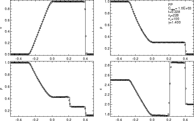
The velocity profiles are shown interactively based on Apache ECharts. Feel free to zoom in/out, check out/in the labels... (It could take some time loading...), but worth waiting. Original code is in shockTubeResults.echart.
Theorem
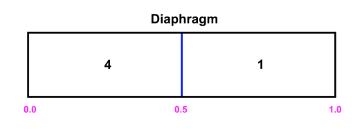
This is an extreme test case used to test solvers, inviscid N-S equations (Euler equations) as shown below brings no diffusion to the system, which makes the problem a nightmare to solvers. \[ \begin{aligned} \frac{\partial \rho}{\partial t}+\nabla \cdot(\rho \mathbf{U}) &=0 \\ \frac{\partial(\rho \mathbf{U})}{\partial t}+\nabla \cdot(\rho \mathbf{U U})+\nabla p &=0 \\ \frac{\partial\left(\rho e_t\right)}{\partial t}+\nabla \cdot\left(\rho e_t \mathbf{U}\right)+\nabla \cdot(p \mathbf{U}) &=0 \\ p &=\rho R_g T \end{aligned} \] It is a Riemann problem with boundary conditions and initial conditions as:
 \[
\begin{aligned}
&\text{All walls are slip} \\
&\mathbf{U}_{\mathbf{4}}=\mathbf{U}_{\mathbf{1}}=0 \\
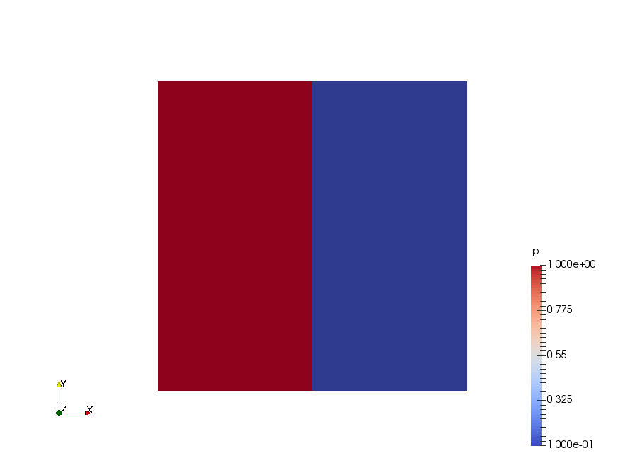
&p_4=1, \quad p_1=0.1 \\
&T_4=0.00348, \quad T_1=0.00278
\end{aligned}
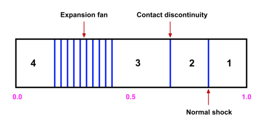
\] Analytical solutions:
\[
\begin{aligned}
&\text{All walls are slip} \\
&\mathbf{U}_{\mathbf{4}}=\mathbf{U}_{\mathbf{1}}=0 \\
&p_4=1, \quad p_1=0.1 \\
&T_4=0.00348, \quad T_1=0.00278
\end{aligned}
\] Analytical solutions:
 |
 |
|---|---|
 |
 |
Result
The velocity profiles are shown below:
From the chart we can see, ignore the fancy TVD methods, there are basically 3 choices of the differencing schemes:
- first-order upwind scheme, no chance to be oscillatory, but very diffusive (smears the solution).
- second-order linear scheme, very accurate but oscillatory. In practice, with complex geometry, the oscillation can lead to an immediate divergence.
- "1.5"-order linearUpwind scheme, usually a good trade off between accuracy and oscillation.
A typical setting for most of the cases in OpenFOAM is:
ddtSchemes
{
  default                         CrankNicolson 0;
}

gradSchemes
{
  default                         cellLimited Gauss linear 1;
  grad(U)                         cellLimited Gauss linear 1;
}

divSchemes
{
  default                         none;
  div(phi,U)                      Gauss linearUpwind grad(U);
  div(phi,omega)                  Gauss linearUpwind default;
  div(phi,k)                      Gauss linearUpwind default;
  div((nuEff*dev(T(grad(U)))))    Gauss linear;
}

laplacianSchemes
{
  default                         Gauss linear limited 1;
}
And also, here is a super stable version, change everything into first-order, it will always push the case to convergence.
ddtSchemes
{
  default                         Euler;
}
gradSchemes
{
  default                         cellLimited Gauss linear 1;
  grad(U)                         cellLimited Gauss linear 1;
}
divSchemes
{
  default                         none;
  div(phi,U)                      Gauss upwind;
  div(phi,omega)                  Gauss upwind;
  div(phi,k)                      Gauss upwind;
  div((nuEff*dev(T(grad(U)))))    Gauss linear;
}
laplacianSchemes
{
  default                         Gauss linear limited 0.5;
}
Note that with linear upwind scheme, we need to specify a method to estimate the gradient. It is always as simple as Gauss linear, (with gradient limiter to avoid overshooting).