Numerical schemes fundamentals 2

Last blog is only 1-equation. In this blog we are going to multi-equation and artificial viscosity.

overview:

Systems of conservation laws

Jacobian matrices, linearised equations, conservative and characteristic variables. Rankine-Hugoniot jump conditions. Boundary conditions.

After dealing with the one-equation task, let's expand to a more general form, recall the 1D inviscid Euler equation in a form of vectors:

Characteristic form

Before moving forward, recall some linear algebra, consider a general 1^st order hyperbolic PDE, \[ \frac{\partial \mathbf{U}}{\partial t}+\mathbf{A}\frac{\partial\mathbf{U}}{\partial x}=0 \] with a square matrix \(\mathbf{A}\),

The PDE is

• linear if \(\mathbf{A} = const\),
• quasi-linear if \(\mathbf{A} = f(\mathbf{U},x,t)\)

The equation is hyperbolic, then \(\mathbf{A}\) is diagonalisable, which means \[ \exists \mathbf{R}: \mathbf{R^{-1} A R=\Lambda}, \quad\text{where } \mathbf{\Lambda} \text{ is diagonal matrix} \] and the diagonal elements \(\lambda_i\) is the eigenvalues / characteristic values of \(\mathbf{A}\), and \(\mathbf{R}\) is a matrix whose columns \(\mathbf{r_i}\) are the right eigenvectors / characteristic vectors of \(\mathbf{A}\). Therefore, multiply by \(\mathbf{R^{-1}}\) both sides of the PDE above to obtain: \[ \mathbf{R^{-1}}\frac{\partial \mathbf{U}}{\partial t}+\mathbf{R^{-1}}\mathbf{A}\frac{\partial\mathbf{U}}{\partial x}=0 \] Define the characteristic variables \(\mathbf{V}\) as \(d\mathbf{V} = \mathbf{R^{-1}}d\mathbf{U}\), we have the characteristic form equation: \[ \begin{aligned} \frac{\partial \mathbf{V}}{\partial t}+\mathbf{R^{-1}}\mathbf{A}\mathbf{R}\frac{\partial\mathbf{V}}{\partial x}=0 \\ \frac{\partial \mathbf{V}}{\partial t}+\mathbf{\Lambda}\frac{\partial\mathbf{V}}{\partial x}=0 \end{aligned} \] It is a wave form and be can decompose the system of PDE into a set of independent equations, such as the \(i^{th}\) equation: \[ \frac{\partial \mathbf{V_i}}{\partial t}+\lambda_i\frac{\partial\mathbf{V_i}}{\partial x}=0 \] so that we can treat the equation as a set (3 for 3D, one for each equation) of independent advection equations, method of characteristics analysis we talked about before can be carried out for each sub-equations. \[ \begin{aligned} \text{Characterstics/wavefronts: } \qquad &dx = \lambda_idt,\\ \text{Characterstic speeds/wave speeds: } \qquad& \lambda_i \end{aligned} \]

So far we have 3 forms:

non-conservative form: no obvious advantage,

conservative form: locate the shock well,

characteristic form: decompose a system of equations into set of independent equations

Euler equation

Its time to introduce the 1D Euler equations: NS equations with 0 viscosity or heat conduction terms:

• Conservation form: \[ \frac{\partial \mathbf{U}}{\partial t}+\frac{\partial \mathbf{F}(\mathbf{U})}{\partial x}=0 \] for the quantity vector \(\mathbf{U}\) with the flux vector \(\mathbf{F}\), \[ \mathbf{U}=\left[\begin{array}{l} \rho \\ \rho u \\ \rho E \end{array}\right] = \left[\begin{array}{l} u_1 \\ u_2 \\ u_3 \end{array}\right] \quad\text{and}\quad \mathbf{F(U)}=\left[\begin{array}{l} \rho u \\ \rho u^{2}+P \\ \rho u\left(E+\frac{P}{\rho}\right) \end{array}\right] = \left[\begin{array}{l} F_1 \\ F_2 \\ F_3 \end{array}\right] \]

• Primitive form: \[ \frac{\partial \mathbf{W}}{\partial t}+\mathbf{C}\frac{\partial \mathbf{W}}{\partial x}=0 \] where: \[ \mathbf{W}=\left[\begin{array}{l} \rho \\ u \\ p \end{array}\right] \quad\text{and}\quad \mathbf{C}=\left[\begin{array}{ccc} u & p & \\ &u & \frac{1}{\rho}\\ & \rho c^2 & u \end{array}\right] \] and \(c=\sqrt{\frac{\gamma p}{\rho}}\), speed of sound.

Characteristic forms of Euler equation

From conservative form

Along with previous method, we can construct the matrix \(\mathbf{A}\) for the conservative Euler equation, \[ \mathbf{A}(\mathbf{U})=\frac{d \mathbf{F}}{d \mathbf{U}}=\left[\begin{array}{ccc} 0 & 1 & 0 \\ \frac{\gamma-3}{2} u^{2} & (3-\gamma) u & \gamma-1 \\ -\gamma u E+(\gamma-1) u^{3} & \gamma E-\frac{3}{2}(\gamma-1) u^{2} & \gamma u \end{array}\right] \] and we have a non-conservation form of the Euler equation, same as the general equation above: \[ \frac{\partial \mathbf{U}}{\partial t}+\mathbf{A}\frac{\partial\mathbf{U}}{\partial x}=0 \]

It is actually non-linear PDE, but we can apply a linear approximation when dealing with small variations around mean values, and the linear approximation form is exactly the same as the non-linear form.

Linear approximation steps:

\(\mathbf{U}\) can be expressed as a constant mean flow \(\mathbf{U_0}\) with a small perturbation \(\mathbf{\tilde{U}}\), substitute the expression into the conservative form of equation: \[\begin{aligned}\frac{\partial \mathbf{(U_0 + \tilde{U})}}{\partial t}+\frac{\partial\mathbf{F(U_0 + \tilde{U})}}{\partial x}=0 \\\frac{\partial \mathbf{U_0}}{\partial t}+\frac{\partial \mathbf{ \tilde{U}}}{\partial t}+\frac{\partial\mathbf{F(U_0 + \tilde{U})}}{\partial x}=0 \\\frac{\partial \mathbf{U_0}}{\partial t}+\frac{\partial \mathbf{ \tilde{U}}}{\partial t}+\frac{\partial\left(\mathbf{F}\left(\mathbf{U}_{0}\right)+\left.\frac{\partial \mathbf{F}}{\partial \mathbf{U}}\right|_{\mathbf{U}_{0}} \tilde{\mathbf{U}}\right)}{\partial x}=0 \\\underbrace{\frac{\partial \mathbf{U_0}}{\partial t}+\frac{\partial\mathbf{F}\left(\mathbf{U}_{0}\right)}{\partial x}}_{0}+\frac{\partial \mathbf{ \tilde{U}}}{\partial t}+\mathbf{\left.A\right|_{U_0}}\frac{\partial\tilde{\mathbf{U}}}{\partial x}=0 \\\end{aligned}\] As a result, with \(\mathbf{A_0=A|_{U_0}}\): \[\frac{\partial \mathbf{ \tilde{U}}}{\partial t}+\mathbf{A_0}\frac{\partial\tilde{\mathbf{U}}}{\partial x}=0\]

With some further tedious calculations, we have \[ \mathbf{R}=\left[\begin{array}{ccc} 1 & \frac{\rho}{2 c} & -\frac{\rho}{2 c} \\ u & \frac{\rho}{2 c}(u+c) & -\frac{\rho}{2 c}(u-c) \\ \frac{u^{2}}{2} & \frac{\rho}{2 c}\left(\frac{u^{2}}{2}+\frac{c^{2}}{\gamma-1}+c u\right) & -\frac{\rho}{2 c}\left(\frac{u^{2}}{2}+\frac{c^{2}}{\gamma-1}-c u\right) \end{array}\right] \] where \(c=\sqrt{\frac{\gamma p}{\rho}}\), speed of sound,

and \(\mathbf{\Lambda}\): \[ \mathbf{\Lambda}=\left[\begin{array}{ccc} u & & \\ &u+c & \\ & & u-c \end{array}\right] \]

From primitive form

The same \(\mathbf{\Lambda}\) can also be obtained by the primitive form of the Euler equation:

We have \(\mathbf{Q^{-1}CQ=\Lambda}\) with， \[ \mathbf{Q}=\left[\begin{array}{ccc} 1 & \frac{\rho}{2 c} & -\frac{\rho}{2 c} \\ 0 & \frac{1}{2} & \frac{1}{2} \\ 0 & \frac{\rho c}{2} & -\frac{\rho c}{2} \end{array}\right] \quad \text { and } \quad \mathbf{Q}^{-1}=\left[\begin{array}{ccc} 1 & 0 & -\frac{1}{c^{2}} \\ 0 & 1 & \frac{1}{\rho c} \\ 0 & 1 & -\frac{1}{\rho c} \end{array}\right] \] Therefore the characteristic equations \(d \mathbf{V}=\mathbf{Q}^{-1} d \mathbf{W}\) become \[ \begin{aligned} &d V_{1}=d \rho-\frac{d p}{c^{2}}=0 \quad &\text{for} \quad \frac{d x}{d t}=u \\ &d V_{2}=d u+\frac{d p}{\rho c}=0 \quad &\text{for} \quad \frac{d x}{d t}=u+c \\ &d V_{3}=d u-\frac{d p}{\rho c}=0 \quad &\text{for}\quad \frac{d x}{d t}=u-c \end{aligned} \] Integrating we get \[ \begin{aligned} &V_{1}=const\quad &\text{for}\quad \frac{d x}{d t}=u \quad(\text { entropy wave) } \\ &V_{2}=u+\int \frac{d p}{\rho c}=const \quad &\text{for} \quad \frac{d x}{d t}=u+c \text { (acoustic wave) } \\ &V_{3}=u-\int \frac{d p}{\rho c}=const \quad &\text{for} \quad \frac{d x}{d t}=u-c \text { (acoustic wave) } \end{aligned} \] These 3 equations can not be solved properly, unless we introduce assumptions.

Closure of Euler equation

For the first equation \(V_1\), we need perfect gas. The equation of state can be used to quantify the specific entropy \(s\) \[ s=c_{v} \ln (p)-c_{p} \ln (\rho) \] with \(c^{2}=\frac{\gamma p}{\rho}\), the ratio of specific heats with \(\gamma=\frac{c_{p}}{c_{v}}\), the constant pressure specific heat \(c_{P}\) and the constant volume specific heat \(c_{v}\). We have \[ d s=-\frac{c_{p}}{\rho}\left(d \rho-\frac{d p}{c^{2}}\right)=-\frac{c_{p}}{\rho} d V_{1} \] \(d V_{1}=0 \Rightarrow\) entropy is constant along a path line \(\frac{d x}{d t}=u\) The other 2 characteristic equations \(V_2, V_3\) can not be analytically integrated, unless further assumptions are made.

For example, assume the flow is homentropic, which means that the entropy is constant everywhere. Inviscid flows are often homoentropic (except at shocks). We have \[ p=A \rho^{\gamma} \quad c=B \rho^{(\gamma-1) / 2} \quad \text { with } \quad \frac{A}{B^{2}}=\frac{1}{\gamma} \] We can show that \(\int \frac{d p}{\rho c}=\frac{2 c}{\gamma-1}+const.\) which lead to \[ \begin{aligned} &S=const &\text{ for }\quad \frac{d x}{d t}=u \text { (entropy wave) } \\ &V_{2}=u+\frac{2 c}{\gamma-1}=const \quad &\text{ for }\quad \frac{d x}{d t}=u+c \text { (acoustic wave) } \\ &V_{3}=u-\frac{2 c}{\gamma-1}=\text { const } \quad &\text{ for } \quad \frac{d x}{d t}=u-c \quad(\text { acoustic wave) } \end{aligned} \] The characteristics \(V_{2}\) and \(V_{3}\) are also known as Riemann invariants. But \(V_{2}\) and \(V_{3}\) have no physical meaning. And this will be a problem in later section.

At this point, the characteristics analysis can be applied, such as:

• Courant number checking
• Rankine-Hugoniot jump condition

Characteristics method of Euler equation

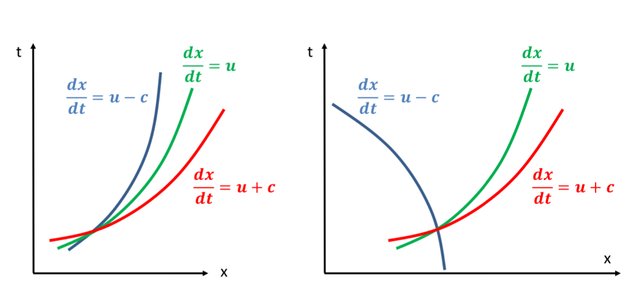
We have three families of characteristics:

1. Characteristics which travel with the local flow speed \(u\)
2. Characteristics which travel with the local flow speed \(+\) the local speed of sound \(u+c\)
3. Characteristics which travel with the local flow speed \(-\) the local speed of sound $u-c $

The signal carried out by acoustic waves does not correspond to any well-known physical quantity. In a supersonic context, all the waves travel in the same direction (it is impossible to have a conversation in supersonic flows). Numerical methods can be easily chose.

In a subsonic context, two wave speeds are positive and one wave speed is negative. That means we have to very carefully to design a numerical scheme considering information from all the directions.

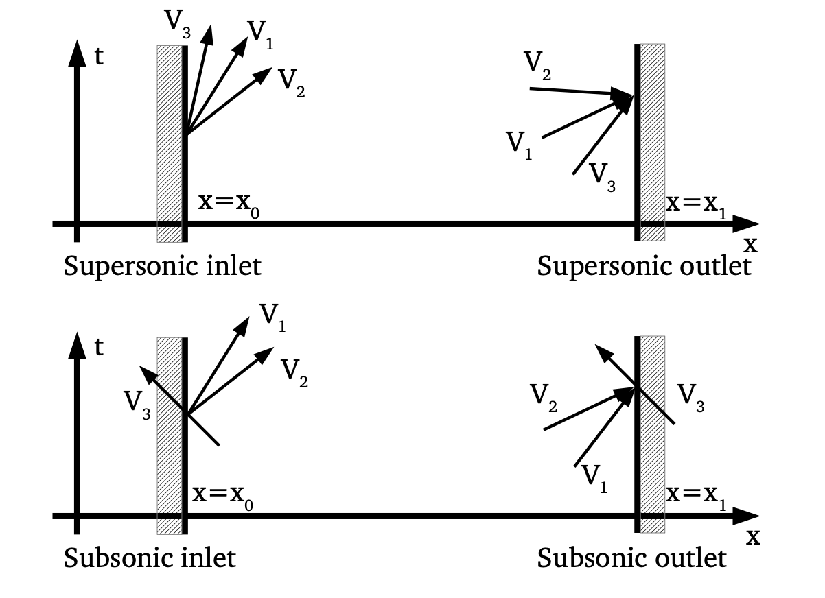
Boundary conditions problem

Given the characteristics in supersonic and subsonic flows, the boundary condition must be carefully designed. As shown below, in the supersonic flow, \(V_1,V_2,V_3\) only need inlet boundary conditions. There is not a big problem. But in the subsonic condition, \(V_1,V_2\) need the inlet boundary conditions, while \(V_3\) needs the outlet boundary condition. Here comes the nightmare. In a subsonic regime, we can't asset the boundary condition for \(V_1,V_2\) and \(V_3\) exactly what they need, because they are non-physical. We don't have direct access of the Riemann variables, the only available conditions are just velocities and pressures. So the characteristic information might have to be defined in an iterative or approximate way

Shock tube solution for Euler equations

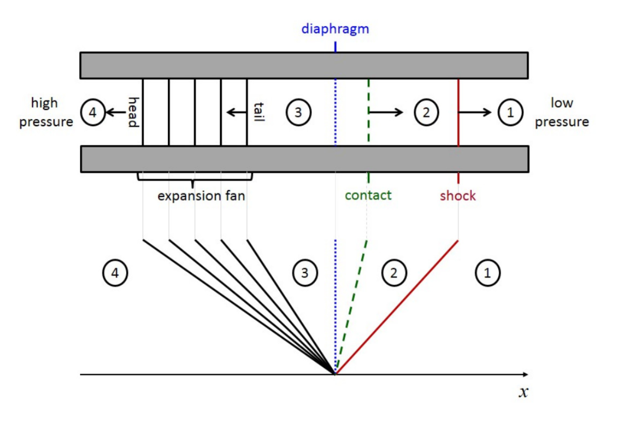
The famous shock tube have 3 regimes:

• Moving shock / shock wave: For the ID Euler equations, the second law of thermodynamics requires that the Mach number \(M = u/c\) must decrease from greater than one to less than one in a coordinate system moving with the shock.

• Centred expansion fan / rarefaction wave: expansion wave in which all characteristics originate from a single point in the \(x—t\) plane

• Contact discontinuity: occurs when the wave speed \(\lambda_1 = u\) and pressure are continuous while other flow properties jump. In other words, for a contact discontinuity \[ u_L=u_R \quad and \quad p_L=p_R \] In multidimensional flows, contact discontinuities are also called slip lines or vortex sheets. Like shocks, contact discontinuities obey the Rankine-Hugoniot relations. Unlike shocks, contacts cannot form spontaneously.

Numerical schemes for non-linear conservation laws

It is still an active research area and these are the classical methods:

Centred schemes: one-step and two-step Lax Wendroff, MacCormack predictor-corrector. Artificial dissipation. Upwind schemes: flux vector and flux difference splitting. Monotone schemes: Godunov and Harten theorems. Exact and approximate Riemann solvers. High-order upwind schemes: the TVD property. The construction of TVD schemes using slope and flux limiters. WENO schemes: weighted essentially non-oscillatory methods

Numerical schemes for Euler equations

Cases to be tested

Case 1: linear advection (\(f(u)=u\)) of a sine wave:

\[ \frac{\partial u}{\partial t}+\frac{\partial u}{\partial x} = 0, \quad \text{with } u(x,0)=-sin(\pi x) \]

Test on \(t=30\), i.e. \(u(x,30)=u(x,0)\)

Case 2: Burger equation (\(f(u)=\frac{1}{2}u^2\)) with Riemann problem,

\[ \frac{\partial u}{\partial t}+\frac{\partial}{\partial x}\left(\frac{1}{2}u^2\right) = 0, \quad \text{with } u(x, 0)=\left\{\begin{array}{ccc} 1 & \text { if } & |x|<\frac{1}{3} \\ -1 & \text { if } & \frac{1}{3}<|x| \leq 1 \end{array}\right. \]

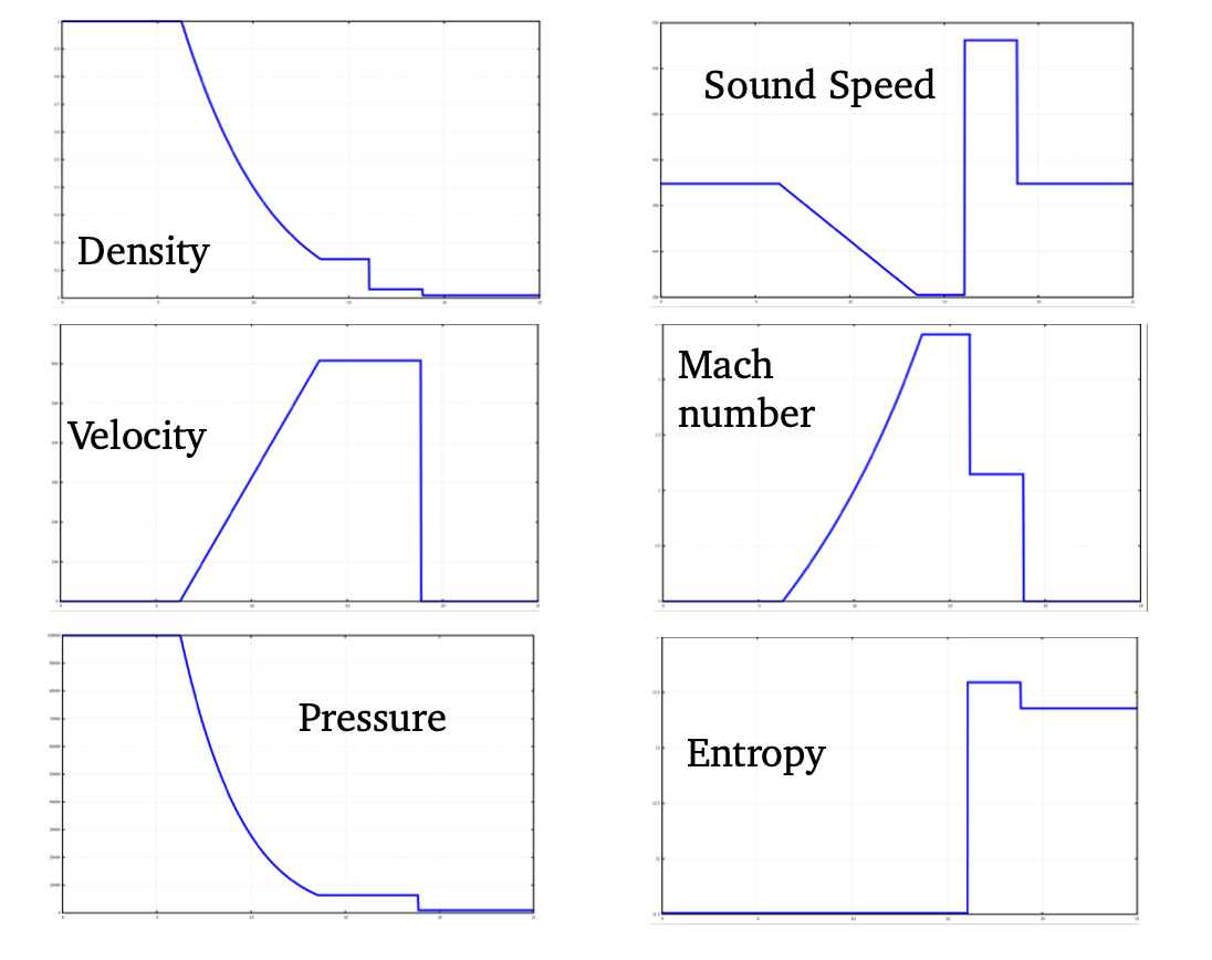
Case 3: Euler equation with Riemann problem

\[ \frac{\partial \mathbf{U}}{\partial t}+\frac{\partial \mathbf{F}(\mathbf{U})}{\partial x}=0 \]

\[ \mathbf{U}=\left[\begin{array}{l} \rho \\ \rho u \\ \rho E \end{array}\right] = \left[\begin{array}{l} u_1 \\ u_2 \\ u_3 \end{array}\right] \quad\text{and}\quad \mathbf{F(U)}=\left[\begin{array}{l} \rho u \\ \rho u^{2}+P \\ \rho u\left(E+\frac{P}{\rho}\right) \end{array}\right] = \left[\begin{array}{l} F_1 \\ F_2 \\ F_3 \end{array}\right] \]

and \(c=\sqrt{\frac{\gamma p}{\rho}}\), speed of sound, \(p=(\gamma-1)\rho(E-\frac{u^2}{2})\). \[ \begin{gathered} \mathbf{W}(x, 0)=\left\{\begin{array}{c} \mathbf{W}_{\mathbf{L}} \text { if } x<0 \\ \mathbf{W}_{\mathbf{R}} \text { if } x \geq 0 \end{array}\right. \\ \mathbf{W}_{L}=\left[\begin{array}{c} \rho_{L} \\ u_{L} \\ p_{L} \end{array}\right]=\left[\begin{array}{c} 1 K g / m^{3} \\ 0 \mathrm{~m} / \mathrm{s} \\ 100,000 \mathrm{~N} / \mathrm{m}^{2} \end{array}\right] \quad \mathbf{W}_{R}=\left[\begin{array}{c} \rho_{R} \\ u_{R} \\ p_{R} \end{array}\right]=\left[\begin{array}{c} 0.010 \mathrm{~kg} / \mathrm{m}^{3} \\ 0 \mathrm{~m} / \mathrm{s} \\ 1,000 \mathrm{~N} / \mathrm{m}^{2} \end{array}\right] \end{gathered} \]

Lax-Friedrichs Method

Recall last time derivation

for case 1 and 2: \[ U^{n+1}_i = \frac{U^n_{i+1}+U^n_{i-1}}{2} - \frac{\Delta t}{\Delta x}\left(\frac{F^n_{i+1}-F^n_{i-1}}{2} \right) \]

for case 3: \[ \begin{gathered} \frac{\partial \mathbf{U}}{\partial t}+\frac{\partial \mathbf{F}(\mathbf{U})}{\partial x}=0 \Rightarrow \frac{\partial \mathbf{U}}{\partial t}+\mathbf{A}(\mathbf{U}) \frac{\partial \mathbf{U}}{\partial x}=0 \\ \mathbf{U}_i^{n+1}=\frac{1}{2}\left(\mathbf{U}_{i+1}^n+\mathbf{U}_{i-1}^n\right)-\frac{\Delta t}{2 \Delta x} \mathbf{\Lambda}\left(\mathbf{U}_{i+1}^n-\mathbf{U}_{i-1}^n\right) \end{gathered} \]

case 1 result

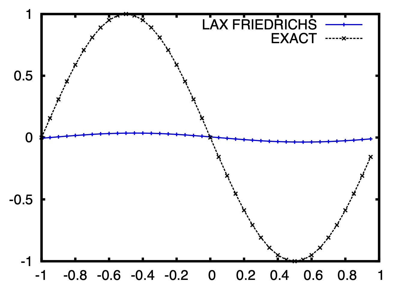
The dissipation effect is huge, but from last blog, we know it can be controlled with higher resolution of \(\Delta x, \Delta t\). (consistent, diffusivity controlled by CFL)

How to control the diffusivity? We can write the scheme in the artificial viscosity form, which will be discussed later.

case 2 result

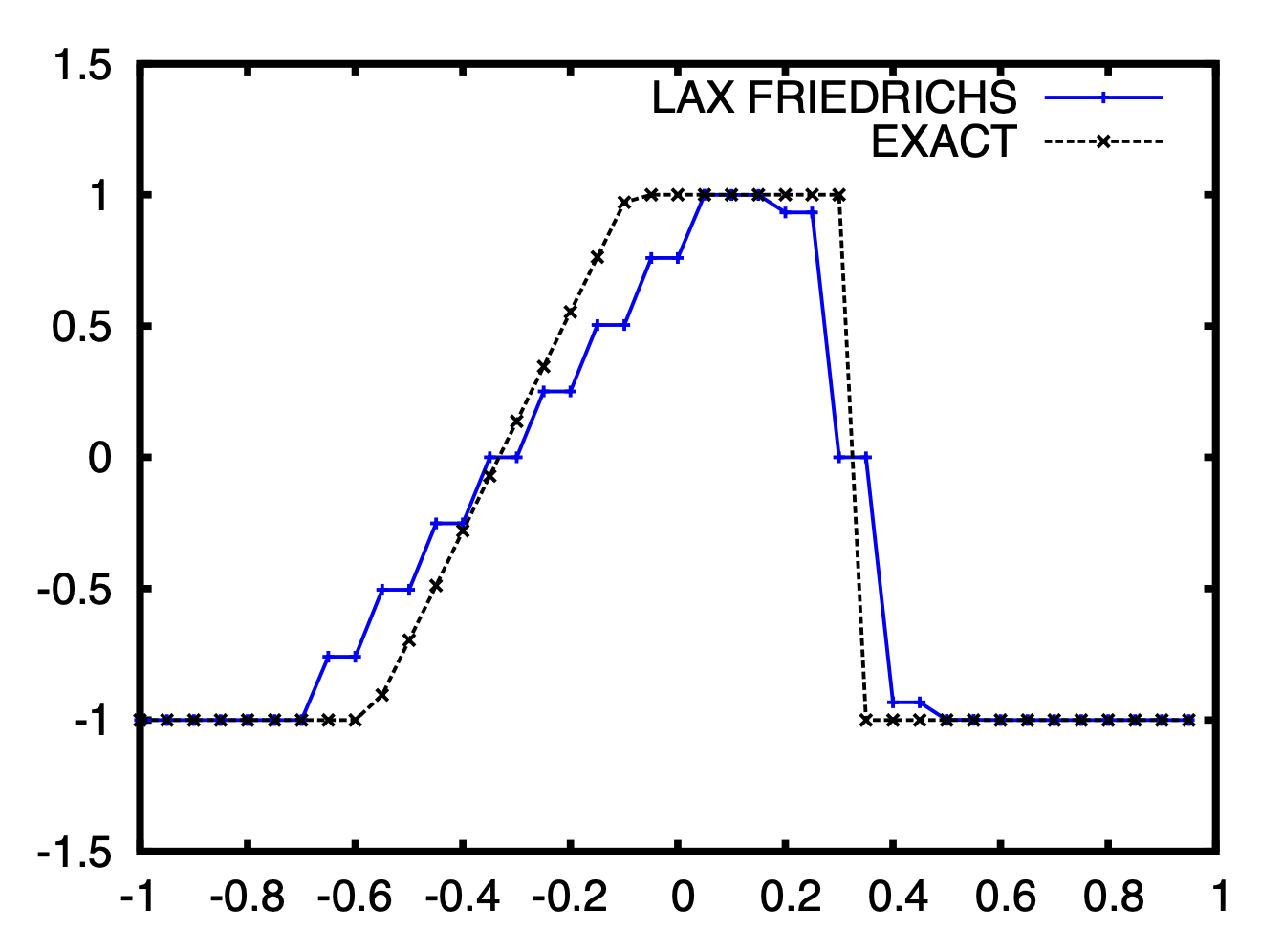
Odd-even oscillations exist, but no over/under shoot.

case 3 results

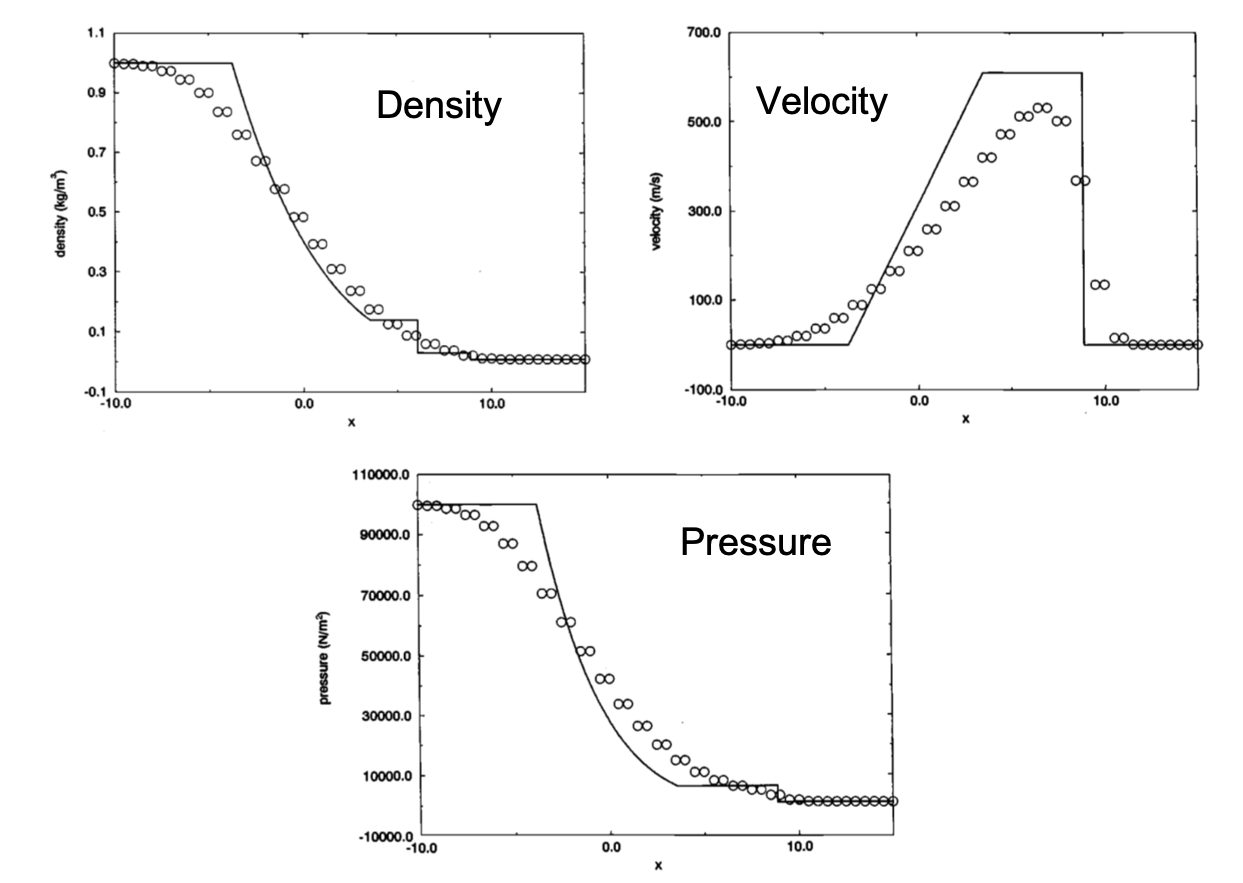
Odd-even oscillations exist. The results are smoothed out. It's difficult to capture the discontinuity of density and pressure. But the results will be fine with increased resolution.

Lax-Wendroff Method

Recall the derivation last time, consider a Taylor serie for \(\mathrm{U}(x, t+\Delta t)\) \[ \mathbf{U}(x, t+\Delta t)=\mathbf{U}(x, t)+\Delta t \frac{\partial \mathbf{U}(x, t)}{\partial t}+\frac{\Delta t^2}{2} \frac{\partial^2 \mathbf{U}(x, t)}{\partial t^2}+O\left(\Delta t^3\right) \] The temporal derivative can be transformed in spatial derivative using the original conservation laws \[ \frac{\partial \mathbf{U}(x, t)}{\partial t}=-\frac{\partial \mathbf{F(U)}}{\partial x} = -\mathbf{A}(\mathbf{U}) \frac{\partial \mathbf{U}}{\partial x}\\ \] \[ \begin{aligned} \frac{\partial^2 \mathbf{U}(x, t)}{\partial t^2}=\frac{\partial}{\partial t}\left(\frac{\partial \mathbf{U}}{\partial t}\right)=-\frac{\partial}{\partial t}\left(\frac{\partial \mathbf{F(U)}}{\partial x}\right) &=-\frac{\partial}{\partial x}\left(\frac{\partial \mathbf{F(U)}}{\partial t}\right) \\ &=-\frac{\partial}{\partial x}\left(\mathbf{A(U)} \frac{\partial \mathbf{U}}{\partial t}\right) \\ &=\frac{\partial}{\partial x}\left(\mathbf{A(U)} \frac{\partial \mathbf{F(U）}}{\partial x}\right) \end{aligned} \] Put the two expressions into the Taylor series, discretise using central differences: \[ \begin{aligned} \mathbf{U}^{n+1}_i=&\mathbf{U}^n_i-\Delta t \frac{\mathbf{F}(\mathbf{U}^n_{i+1})-\mathbf{F}(\mathbf{U}^n_{i-1})}{2\Delta x}+ \\ &\frac{\Delta t^2}{2} \frac{\mathbf{A}_{i+1 / 2}^n\frac{\mathbf{F}(\mathbf{U}^n_{i+1})-\mathbf{F}(\mathbf{U}^n_{i})}{\Delta x} -\mathbf{A}_{i-1 / 2}^n\frac{\mathbf{F}(\mathbf{U}^n_{i})-\mathbf{F}(\mathbf{U}^n_{i-1})}{\Delta x}} {\Delta x^2} \end{aligned} \] There are two choice of defininig \(\mathbf{A}_{i+1 / 2}^n\), \(\mathbf{A}\left(\mathbf{U}_{i+\frac{1}{2}}^n\right)\) or \(\frac{1}{2}\left(\mathbf{A}_i^n+\mathbf{A}_{i+1}^n\right)\), taking \(\mathbf{U}_{i+\frac{1}{2}}\) to calculate \(\mathbf{A}\) or average \(\mathbf{A}\) from the its neighbouring time steps.

Recall that \(\mathbf{A}\) is a matrix with 9 elements, and it is a function of \(x\) and \(t\). i.e. \(\mathbf{A}\) updates with every time step at every nodes. And this will lead to a cost problem

In the Lax-Wendroff method, the average wave speeds \(\mathbf{A}_{i+1 / 2}^n\) may be defined in a variety of different ways. It is actually an entire class of methods depending on the choice of the wave speeds.

Furthermore, we write the Lax-Wendroff method in conservation form: \[ \mathbf{U}_i^{n+1}=\mathbf{U}_i^n-\frac{\Delta t}{\Delta x}\left(\mathbf{F}_{i+\frac{1}{2}}^n-\mathbf{F}_{i-\frac{1}{2}}^n\right) \] with \[ \mathbf{F}_{i+\frac{1}{2}}^n=\frac{\mathbf{F}\left(\mathbf{U}_i^n\right)+\mathbf{F}\left(\mathbf{U}_{i+1}^n\right)}{2}-\frac{\Delta t}{2 \Delta x} \mathbf{A}_{i+\frac{1}{2}}^n\left(\mathbf{F}\left(\mathbf{U}_{i+1}^n\right)-\mathbf{F}\left(\mathbf{U}_i^n\right)\right) \] for case1 and 2, the linear advection equation, \(f(u)=a u\) it takes the form \[ u_i^{n+1}=u_i^n-\frac{\sigma}{2}\left(u_{i+1}^n-u_{i-1}^n\right)+\frac{\sigma^2}{2}\left(u_{i+1}^n-2 u_i+u_{i-1}^n\right) \] where \(\sigma=a \frac{\Delta t}{\Delta x}\). The corresponding conservative flux is \[ F_{i+\frac{1}{2}}^n=a \frac{u_i^n+u_{i+1}^n}{2}-\frac{\Delta t}{2 \Delta x} a^2\left(u_{i+1}^n-u_i^n\right) \]

case 1 result

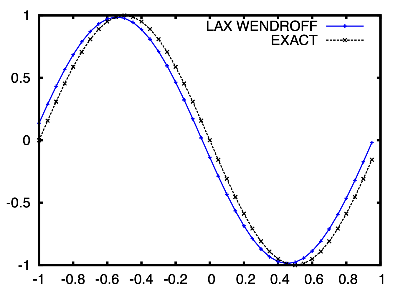
The Lax Wendroff result slightly shifted (delay), because the schemes is not consistent as discussed in last blog. It can beed seen that the Lax Wendroff method is not suitable for simple non-discontinue problems.

case 2 result

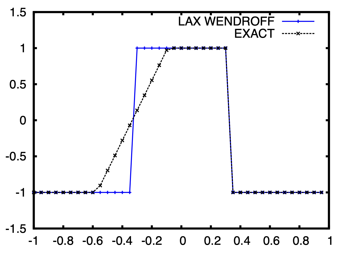
Here the rarefaction wave is not captured, WRONG SOLUTION! As discussed before, the conservation form locates the shock perfectly but the result cannot be guaranteed as physical. And it is not suitable for system of conservation.

There is no need to test case 3 because we know it will have a slight delay, and wrong solution.

Two-step Lax-Wendroff Method (Richtmyer method)

This is an optimisation of Lax-Wendroff. The idea is to reduce the cost by the \(\mathbf{A}\) matrix

There are two options:

• Option 1: Approximate matrix \(\mathbf{A}\): Still too expensive.
• Option 2: Avoid computation of matrix \(\mathbf{A}\) (Jacobian free methods): Richtmyer method introducing intermedia time steps \(n+\frac{1}{2}\) as follows

Step 1 \[ \begin{aligned} &\mathbf{U}_{i+1 / 2}^{n+1 / 2}=\frac{1}{2}\left(\mathbf{U}_{i+1}^n+\mathbf{U}_i^n\right)-\frac{\Delta t}{2 \Delta x}\left(\mathbf{F}\left(\mathbf{U}_{i+1}^n\right)-\mathbf{F}\left(\mathbf{U}_i^n\right)\right) \\ &\mathbf{U}_{i-1 / 2}^{n+1 / 2}=\frac{1}{2}\left(\mathbf{U}_i^n+\mathbf{U}_{i-1}^n\right)-\frac{\Delta t}{2 \Delta x}\left(\mathbf{F}\left(\mathbf{U}_i^n\right)-\mathbf{F}\left(\mathbf{U}_{i-1}^n\right)\right) \end{aligned} \] Step 2 \[ \mathbf{U}_i^{n+1}=\mathbf{U}_i^n + \Delta t \frac{\partial\mathbf{U}_{i}^{n+1 / 2}}{\partial t} = \mathbf{U}_i^n-\Delta t\frac{\partial\mathbf{F}_{i}^{n+1 / 2}}{\partial x} = \mathbf{U}_i^n-\frac{\Delta t}{\Delta x}\left[\mathbf{F}\left(\mathbf{U}_{i+1 / 2}^{n+1 / 2}\right)-\mathbf{F}\left(\mathbf{U}_{i-1 / 2}^{n+1 / 2}\right)\right] \] Conservative form are used to avoid the calculation of \(\mathbf{A}\) matrix.

• This first step is called the predictor (here Lax-Friedriechs method)
• The second step is called the corrector (here Leapfrog method)

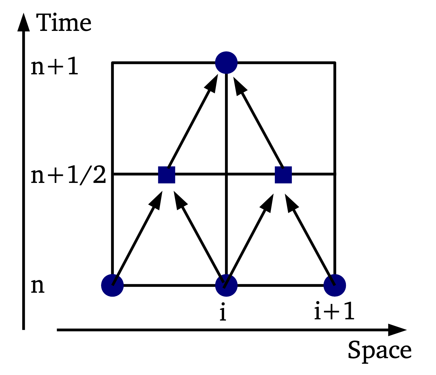
The idea is inspired from the Two-step runge–kutta methods for ordinary differential equations. Apart from the standard grid \(x_i\); another the staggered grid \(x_{i+ 1/2} = (x_{i+1} + x_i )/2\) lies halfway between the standard grid points.

Staggered grids are extremely common in predictor-corrector methods.

case 3 results

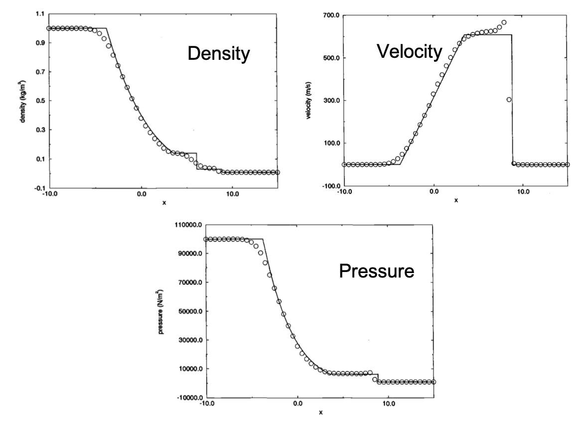
The result is highly diffusive on the shock. For velocity, although the shock and rarefaction wave are captured, oscillations exist because of the second order. For pressure, a slight overshoot also exit on the upstream of the shock.

Note the scheme is upwind, so if there is a bidirectional supersonic flow, this scheme will not work well.

Two-step MacCormack’s method

This is another variance of the two step lax wandroff method, and it is one of the most used method for compressible flow.

The idea is to combine upwind and downwind method so that the bidirectional supersonic wave can be evaluated well.

Predictor step: 1^st order upwind (first guess) \[ \mathbf{U}_i^*=\mathbf{U}_i^n-\frac{\Delta t}{\Delta x}\left(\mathbf{F}\left(\mathbf{U}_{i+1}^n\right)-\mathbf{F}\left(\mathbf{U}_i^n\right)\right) \] Corrector step: 1^st order down wind \[ \mathbf{\hat U}_i= \mathbf{U}_i^* + \Delta t \frac{\partial\mathbf{U}_i^*}{\partial t}= \mathbf{U}_i^* - \Delta t \frac{\partial\mathbf{F}(\mathbf{U}_i^*)}{\partial t} =\mathbf{U}_i^*-\frac{\Delta t}{\Delta x}\left[\mathbf{F}\left(\mathbf{U}_i^*\right)-\mathbf{F}\left(\mathbf{U}_{i-1}^*\right)\right] \] Finally step, average \[ \mathbf{U}_i^n = (\mathbf{\hat{U}}_{i}+\mathbf{U}_{i}^{*})/2 \] The predictor and corrector in MacCormack’s method can be reversed depending if we have left-running or right-running waves. The two versions of MacCormack’s method are often combined to a mix of left and right running waves.

The predictor or corrector are both unconditionally unstable, yet the sequence is stable if \(CFL<1\).

The MacCormack’s method is still second order although two two steps are first order.

Even with the sophisticated methods available today, many people still turn to MacCormack’s method first, especially in the absence of shocks, mainly because of its simplicity and efficiency.

case 3 result

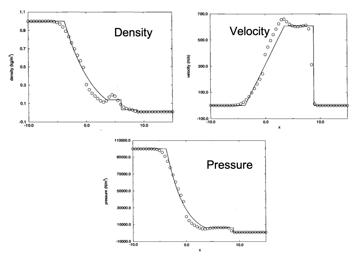
Oscillation with shocks because the second order.

Artificial viscosity

Artificial viscosity for Scalar Conservation Law

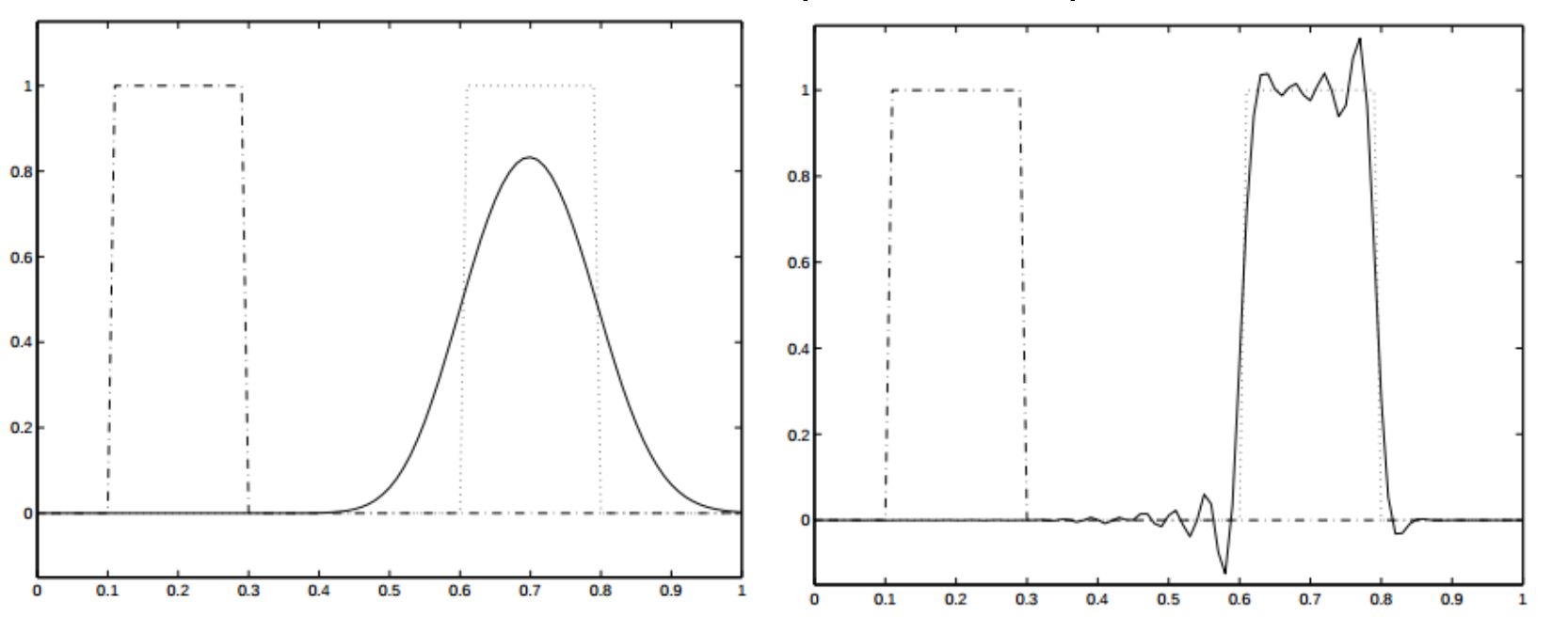
Firstly, recall the difference between diffusion and dispersion. Diffusion(left) means the smearing effect with convection, while dispersion(right) represents the effect of oscillation. We are seeking a method to control the balance of diffusion and dispersion of a numerical method.

The idea of artificial viscosity is that, there is no viscous terms in Euler equations but we can have some viscous effect (diffusive effects) inside numerical methods.

For example, a scalar conservation law with a viscous-like term (like in N-S): A conservative forward \[ \frac{\partial u}{\partial t}+\frac{\partial f(u)}{\partial x}=\frac{\partial}{\partial x}\left(d(u) \frac{\partial u}{\partial x}\right)\\ \] where \(d(u)\) is the viscous term and it should be as small as possible. Besides, unlike the constant real viscosity in the N-S, \(d\) can be non-constant locally.

Use central difference to discretise this formula as: \[ \frac{u_i^{n+1}-u_i^n}{\Delta t}+\frac{f\left(u_{i+1}^n\right)-f\left(u_{i-1}^n\right)}{2 \Delta x}=\frac{d_{i+1 / 2} \frac{u_{i+1}^n-u_i^n}{\Delta x} - d_{i-1 / 2} \frac{u_i^n-u_{i-1}^n}{\Delta x}}{\Delta x} \]

A oscillatory scheme can be controlled by introducing diffusion, i.e. artificial viscosity.

Artificial Viscosity Form

Take The Lax-Friedrich's method as an example, the conservative form can be written in the artificial viscosity form.

Non-conservative form: \[ u_i^{n+1}=\frac{1}{2}\left(u_{i-1}^n+u_{i+1}^n\right)-\frac{\Delta t}{2 \Delta x}\left[f\left(u_{i+1}^n\right)-f\left(u_{i-1}^n\right)\right] \] Conservative form: \[ u_i^{n+1}=u_i^n-\frac{\Delta t}{\Delta x}\left[F_{i+1 / 2}^n-F_{i-1 / 2}^n\right]$ with $F_{i+1 / 2}^n=\frac{\Delta x}{2 \Delta t}\left(u_i^n-u_{i+1}^n\right)+\frac{1}{2}\left[f\left(u_i^n\right)+f\left(u_{i+1}^n\right)\right] \]

Artificial viscosity form: \[ u_i^{n+1}=u_i^n-\frac{\Delta t}{2 \Delta x}\left[f\left(u_{i+1}^n\right)-f\left(u_{i-1}^n\right)\right]+\frac{\Delta t}{2 \Delta x}\left[d_{i+1 / 2}\left(u_{i+1}^n-u_i^n\right)-d_{i-1 / 2}\left(u_i^n-u_{i-1}^n\right)\right] \] with \(d_{i+1 / 2}=\frac{\Delta x}{\Delta t}\),

Most of the schemes can be written in artificial viscosity form so that one can quantify the diffusivity by inspecting the \(d_{i+1 / 2}\). We can as a result analysis, then control the diffusivity of a scheme.

For example for Lax-Friedrich's method:

• reduce $x $, the diffusivity will be reduced.

• reduce \(\Delta t\) the diffusivity will be increased.

The dissipation can be easily controlled by increasing the space resolution, or selecting the highest possible CFL number.

Some points:

• The discretisation of this term does not need to be acurate; all we want is to have desirable numerical effects.
• Implicit artificial viscosity: arises naturally as part of the discretisation of the first derivative.
• Explicit artificial viscosity: added on purpose to remove oscillations.

Artificial Viscosity for System of Conservation Laws

For systems of conservation laws, the artificial dissipation term can be considered a discretisation of \[ \frac{\partial}{\partial x}\left(\mathbf{D(u)} \frac{\partial \mathbf{U}}{\partial x}\right)\\ \] where \(\mathbf{D}\) is used to add explicit artificial dissipation on the scheme to control the high-frequency oscilations. This is analogous to \[ \frac{\partial}{\partial x}\left(d(u) \frac{\partial u}{\partial x}\right)\\ \]

for scalar conservation laws as seen in previous subsection.

Requirement for artificial dissipation

The (explicit) dissipation matrix \(\mathbf{D}\) should satisfy:

• The dimensions of \(\mathbf{D}\) are those of \(\mathbf{A}\).
• Its influence in smooth regions should be negligible. It should act only around discontinuities (i.e in areas with strong gradients).
• It should be non-linear, i.e. depends on \(\mathbf{U}\)
• \(\mathbf{D}\) should be proportional to, at least, \(\Delta x\) in order to maintain second-order accuracy.
• Different schemes may need different levels of dissipation.
• Explicit artificial dissipation terms are added to the numerical flux.

For example, the Richtmyer method with this sort of artificial viscosity becomes

Step 1, not changed \[ \begin{aligned} &\mathbf{U}_{i+1 / 2}^{n+1 / 2}=\frac{1}{2}\left(\mathbf{U}_{i+1}^n+\mathbf{U}_i^n\right)-\frac{\Delta t}{2 \Delta x}\left(\mathbf{F}\left(\mathbf{U}_{i+1}^n\right)-\mathbf{F}\left(\mathbf{U}_i^n\right)\right) \\ &\mathbf{U}_{i-1 / 2}^{n+1 / 2}=\frac{1}{2}\left(\mathbf{U}_i^n+\mathbf{U}_{i-1}^n\right)-\frac{\Delta t}{2 \Delta x}\left(\mathbf{F}\left(\mathbf{U}_i^n\right)-\mathbf{F}\left(\mathbf{U}_{i-1}^n\right)\right) \end{aligned} \] Step 2, add artificial viscosity \[ \mathbf{U}_i^{n+1}= \mathbf{U}_i^n-\frac{\Delta t}{\Delta x}\left[\mathbf{F}\left(\mathbf{U}_{i+1 / 2}^{n+1 / 2}\right)-\mathbf{F}\left(\mathbf{U}_{i-1 / 2}^{n+1 / 2}\right)\right] +d[\mathbf{U}_{i+1}^n-\mathbf{U}_{i}^n+\mathbf{U}_{i-1}^n] \] But both Richtmyer and MacCormack’s methods remain oscillate with artificial viscosity.

• For the Euler equations, without artificial viscosity, neither MacCormack’s method nor the Richtmyer method can complete the first time step without overshooting and creating negative pressures.
• Both methods take two time steps with a constant coefficient of second-order artificial viscosity d = 0.02. After the first two time steps have smoothed the initial conditions, both methods are able to continue without artificial viscosity.
• Overshoots and oscillations without continued use of artificial viscosity.