Numerical schemes fundamentals

This is the essence of CFD, advecting with the discontinuities due to inviscid fluid PDEs. Several computational schemes are introduced with fortran scripts.

This is a revise of my graduate CFD course and fortran. The aim is to further the understanding of finite volume method and the fvscheme dict in OpenFOAM. But in this blog finite difference method is used all the time for the simplicity.

Reference books:

E.F. Toro, Riemann Solvers and Numerical Methods for Fluid Dynamics, Springer-Verlag.

R.J. LeVeque, Finite Volume Methods for Hyperbolic Problems, Cambridge University Press.

Overview:

Scalar conservation laws

1-D theory. Examples of 1-D hyperbolic conservation laws. Characteristics discontinuities and jump conditions. Weak solutions and entropy condition. Linear versus non-linear advection

Challenges

As we all know, flow fluids are governed by 3 hyperbolic PDEs (conservation of mass, momentum and energy). These equations are highly non-linear and they can lead to discontinuities even with a smooth initial conditions, which is very difficult to solve numerically. Simple FDM will definitely fail on these discontinuities and shocks.

Recall the incompressible NS equation that we've learned in the kindergarten: \[ \frac{\partial \mathbf{V}}{\partial t} + \underbrace{\left(\boldsymbol{\nabla}\cdot\mathbf{V}\right)\mathbf{V}}_{\text{convection}} = \frac{\nabla p}{\rho} + \mathbf{g}+ \underbrace{\nu \boldsymbol{\nabla}^2\mathbf{V}}_{\text{diffusion}} \] the viscous diffusion term in the equation leads to parabolic equations with smooth solutions, which will save our life. But with very high \(Re\), the equation reduces to pure hyperbolic inviscid Euler Equation, and the resultant discontinuity is a nightmare for most of the numerical schemes.

The presence of discontinuities requires weak solutions, as oppose to strong solutions.

However, the weak solutions give up the uniqueness in math, i.e there exist a large number of solutions that may not be physical acceptable, i.e. extra conditions are needed to justify the solution. They are:

• Rankine-Hugoniot condition deals with the discontinuity
• Entropy condition satisfies the physics

Just here to remind that we are dealing with inviscid flow, shocks, nothing to do with turbulence.

Scalar conservation law

1D law

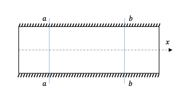
First let's introduce a simple example to present the problem: consider an 1D control volume \([a,b]\), during the time interval \([t_1,t_2]\) . The scalar conservation law can be stated as that during \([t_1,t_2]\) , change in total conserved quantity in \([a,b]\) equals the net flux through the boundaries \(a\), \(b\):

\[ \frac{d}{dt}\int_a^bu(x,t) = -\left[f(u(b,t))-f(u(a,t))\right] \] where \(u(x,t)\) is called the conserved quantity while \(f\) denotes the flux. This equation often describes the transport phenomena.

You can not create, you can not destroy.

Integral, differential conservative and primitive forms

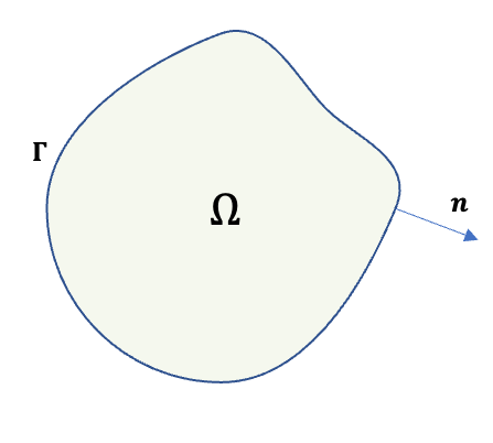
The 1D law can be extended in 2D with the relation, in integral form. \[ \frac{d}{d t} \int_{\Omega} \mathbf{u} d \Omega+\int_{\Gamma} \mathbf{f}(\mathbf{u}) \cdot \mathbf{n} d \Gamma=0 \]

The FVM and FEM solves the integral form, while the FDM solves the primitive form.

Apply the Gauss divergence theorem the relation can be represented as differential form: \[ \begin{aligned} \int_{\Omega}\left\{\frac{\partial \mathbf{u}}{\partial t}+\nabla \cdot \mathbf{f}(\mathbf{u})\right\} d \Omega=0& \\ \Rightarrow \color{purple}{ \forall \Omega,\quad \frac{\partial \mathbf{u}}{\partial t}+\nabla \cdot \mathbf{f}(\mathbf{u})=0} & \end{aligned} \] above is called the differential conservative form. The only \(u\) changed in time is due to the flux \(f\). There is no extra assumptions introduced.

In comparison, with an assumption of \(\mathbf{a} = \frac{d\mathbf{f}}{d\mathbf{u}}\), the equation can be rewritten with the chain rule, as the differential primitive form : \[ \quad \frac{\partial \mathbf{u}}{\partial t}+\mathbf{a}(\mathbf{u})\nabla \cdot \mathbf{u}=0, \quad \text{where }\mathbf{a} = \frac{d\mathbf{f}}{d\mathbf{u}} \] This form is identical to above in mathematics, but it will lead to problems numerically when dealing with discontinuities (to be discussed later).

Rankine-Hugoniot Jump condition

When dealing with discontinuities, the integral form is well defined, but not the differential forms. The differential solvers can't deal with the drastic derivatives so instead they solve an extra jump condition which can be derived from the well-defined integral form (discussed later).

For an 1D jump discontinuity travelling at the speed \(s\): \[ f(u_r)-f(u_l) = s(u_r-u_s) \] where \(u_r\), \(u_l\) represent the speeds just at the left and the right of the discontinuity.

1D Euler equations

Its time to introduce the 1D Euler equations: NS equations with 0 viscosity or heat conduction terms: \[ \frac{\partial}{\partial t}\left[\begin{array}{l} \rho \\ \rho u \\ \rho E \end{array}\right]+\frac{\partial}{\partial x}\left[\begin{array}{l} \rho u \\ \rho u^{2}+P \\ \rho u\left(E+\frac{P}{\rho}\right) \end{array}\right]=0 \] And the conservation form is: \[ \frac{\partial \mathbf{q}}{\partial t}+\frac{\partial \mathbf{F}(\mathbf{q})}{\partial x}=0 \] for the quantity vector \(\mathbf{q}\) with the flux vector \(\mathbf{F}\).

Conservation vs non-conservation form

Similar to before, with terms in a form of \(\partial_x{uv}\): \[ \frac{\partial uv}{\partial x} \neq u\frac{\partial v}{\partial x}+ v\frac{\partial u}{\partial x} \] When dealing with the discontinuities, the conservative LHS locates the shock directly, while the non-conservative RHS does not. (to be discussed later)

Close the Euler equation

Unlike the well-posed NS equation, in Euler equation, we have 4 unknowns but only 3 equations. So an extra state equation, i.e. extra assumption of the gas state is needed. Sometimes it's the idea gas assumption \(p = \rho RT\), but for high \(Re\) compressible flows, equations of state are required to describe the relation between \(p, \rho \text{ and }T\).

We are going to use the 1D Euler equations to evaluate the numerical methods.

Analytical solutions of Euler equations

Linear Advection Equation

In 1D, the linear advection law for \(u(x,t)\) is: \[ \color{purple} \frac{\partial u }{\partial t} + a(u)\frac{\partial u }{\partial x} = 0 \] where \(a(u)\) denotes the advection speed. Plus an initial condition \(u(x,0)\) and boundary condition (discuss later).

solution

This is a simple 2-variable PDE and we can apply the method of characteristics:

1. Imagine a characteristic line \(s\), we have the chain rule: \[ \frac{d u(x,t)}{d s} = \frac{d t}{d s}\frac{\partial u}{\partial t} + \frac{d x}{d s} \frac{\partial u}{\partial x} \]

2. As a result we can construct, \[ \begin{aligned} \frac{d u(x,t)}{d s} = 0,\quad\frac{d t}{d s}=1, \quad \frac{d x}{d s}= a \\ \Rightarrow \quad \frac{d u}{0}=\frac{d t}{1}=\frac{d x}{a}= d s \end{aligned} \]

3. Select the available equations we have the characteristic equation: \[ \begin{aligned} \frac{d x}{d t} &= a \\ \Rightarrow\quad x &= x_0 + a(u)t \end{aligned} \] If \(u(x_0,0)=u_0\), then \(\frac{dx}{dt}=a(u_0)\), the characteristic equation is therefore: \[ \color{purple} x = x_0 + a(u_0)t \]

4. And the solution to the problem is: \[ u(x,t) = f(x_0) = f(x-a(u_0)t) \]

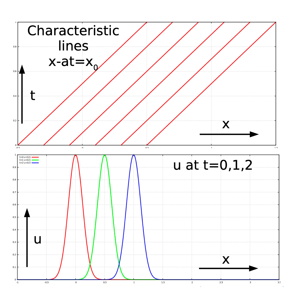
Linear Advection Equation Example

Solve the following advection equation where \(a = 0.5\) \[ \frac{\partial u}{\partial t} + a \frac{\partial u}{\partial x }= 0 \] with initial condition \[ u(x,0) = exp(-32x^2) \]

solution

The characteristics are straight lines in the \((x,t)\) plane: \[ x = 0.5t+x_0 \] And the solutions are therefore: \[ u(x,t) = f(x_0) = exp(-32(x-0.5t)^2) \]

Inviscid Burgers' equation

In 1D, the inviscid Burgers' equation for \(u(x,t)\) is: \[ \color{purple} \frac{\partial u }{\partial t} + \frac{f(u) }{\partial x} = 0,\quad\text{where }f(u)=\frac{1}{2}u^2 \] The conservative form for this equation： \[ \frac{\partial u }{\partial t} + \frac{\partial(\frac{1}{2}u^2) }{\partial x} = 0 \] and the primitive form: \[ \frac{\partial u }{\partial t} + u\frac{\partial u }{\partial x} = 0 \] same form as the 1D linear advection equation with \(a(u)=u\).

Burgers' equation Example

Solve the advection equation: \[ \frac{\partial u}{\partial t} + u \frac{\partial u}{\partial x }= 0 \] with initial condition: \[ u(x,0) = 1-\cos(x) \]

solution

Similarly, the characteristics are described by: \[ x = x_0 + ut \] and the solution: \[ u = 1-\cos(x-ut) \] which is implicit. It is can be plotted anyway:

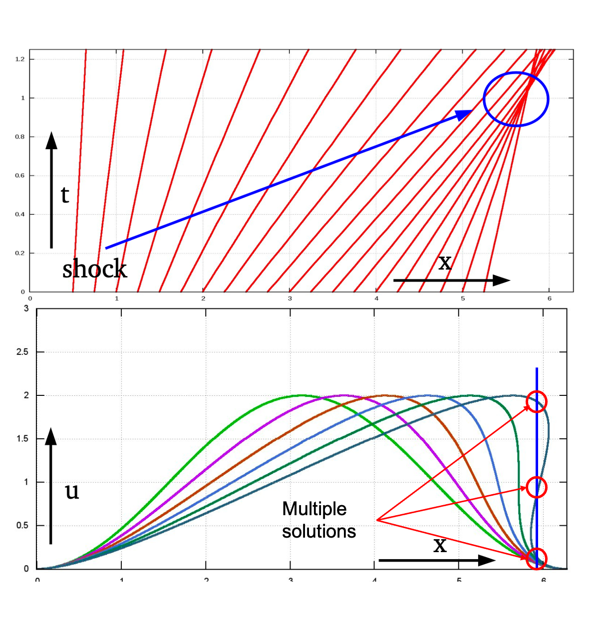
discussion

For non-linear conservation laws, the characteristics may cross within finite time. This would suggest a multi-valued solution which does not make sense physically.

Where the characteristics start crossing, the solution become discontinuous. And the formation of discontinuities is possible even for smooth initial data. So the differential primitive form of the equations is no longer valid

\(\Rightarrow\) only the integral form can deal with discontinuities. And the differential form can be completed by a jump condition derived from the integral form.

\(\Rightarrow\) we need weak solutions. The mathematical theory of partial differential equations introduces the concept of weak solutions.

Rankine-Hugoniot condition

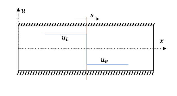
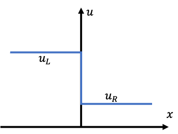
The Riemann Problem

In order to understand the behaviour of the solution at discontinuities, it is useful to start with a simplified problem.

The Riemann problem is a conservation law with a single discontinuity. \[ \color{purple} \frac{\partial u}{\partial t} + \frac{\partial f(u)}{\partial x} = 0 \] with \[ \color{purple} u(x, 0)= \begin{cases}u_{L} & x \leq 0 \\ u_{R} & x>0\end{cases} \]

Shock Path

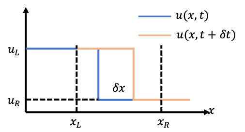
Take the control volume between boundaries \(x_L\) and \(x_R\), which are taken sufficient close to the shock so that spatial variations of the solution become unimportant. and are taken sufficient apart from the shock so that the boundary will note interfere with the shock motion over time interval \(\delta t\).

Recall the integral function: \[ \frac{d}{dt}\int_{x_L}^{x_R}udx = f(u_L)-f(u_R) \] If the position of the shock is \(x = X(t)\), with \(x_L< X (t) <x_R\), the values of \(u(x,t)\) inside the integral are close to the constants \(u_L\) and \(u_R\) and we can write: \[ \begin{aligned} \frac{d}{dt}\int_{x_L}^{X}u_Ldx + \frac{d}{dt}\int_{X}^{x_R}u_Rdx= f(u_L)-f(u_R)\\ \frac{d}{dt}\left[(x_L-X)u_L + (X-x_R)u_R\right]= f(u_L)-f(u_R)\\ \end{aligned} \]

Given the shock speed (slope of the shock path) \(s = \frac{dX}{dt}\), we have: \[ \begin{aligned} s\left(u_L - u_R\right)&= f(u_L)-f(u_R)\\ \color{purple} s= \frac{dX}{dt}&\color{purple} = \frac{f(u_L)-f(u_R)}{\left(u_L - u_R\right)}= \frac{f(u_R)-f(u_L)}{\left(u_R - u_L\right)} \end{aligned} \] The equation above is the Rankine-Hugoniot condition, also called the "jump condition".

Correspondingly, weak solutions represents the solutions of the PDE where the solution is smooth and of a Rankine-Hugoniot condition at discontinuities. And they are not unique.

Strong solution \(\Rightarrow\) weak solution

Weak solution \(\nLeftarrow\) Strong solution

Non-uniqueness of weak solutions

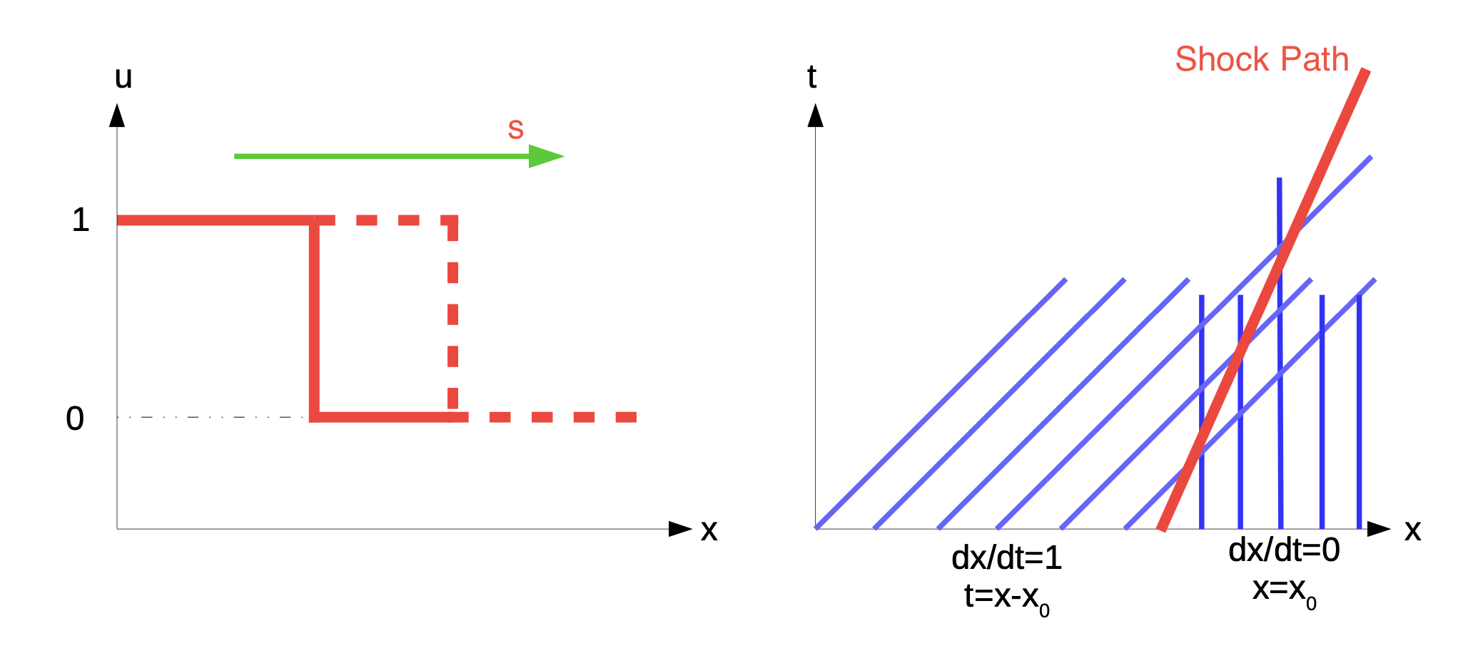
Example of Riemann Problem with Burgers's equation

Consider the Burgers' equation under a Riemann Problem: \[ \begin{aligned} \frac{\partial u}{\partial t} + u \frac{\partial u}{\partial x }&= 0, \\ \text{with } u(x, 0)&= \begin{cases}1 & x \leq 0 \\ 0 & x>0\end{cases} \end{aligned} \] The characteristics are of the form: \(x = x_0 + ut\)

In \(x-t\) plane, the characteristics line: \[ \begin{cases} x = t - x_0 & x_0 \leq 0 \\ x = x_0 & x_0 > 0\end{cases} \] And the according to the Rankine-Hugonoit condition, the speed of the shock is: \[ s = \frac{f(u_L)-f(u_R)}{\left(u_L - u_R\right)}= \frac{-1/2-0}{\left(1-0\right)} = \frac{1}{2} \] and the shock path is: \[ x = \frac{1}{2} t \] therefore, the solution is: \[ u(x,t) = \begin{cases} 1 & x \leq \frac{1}{2}t \\ 0 & x> \frac{1}{2}t\end{cases} \]

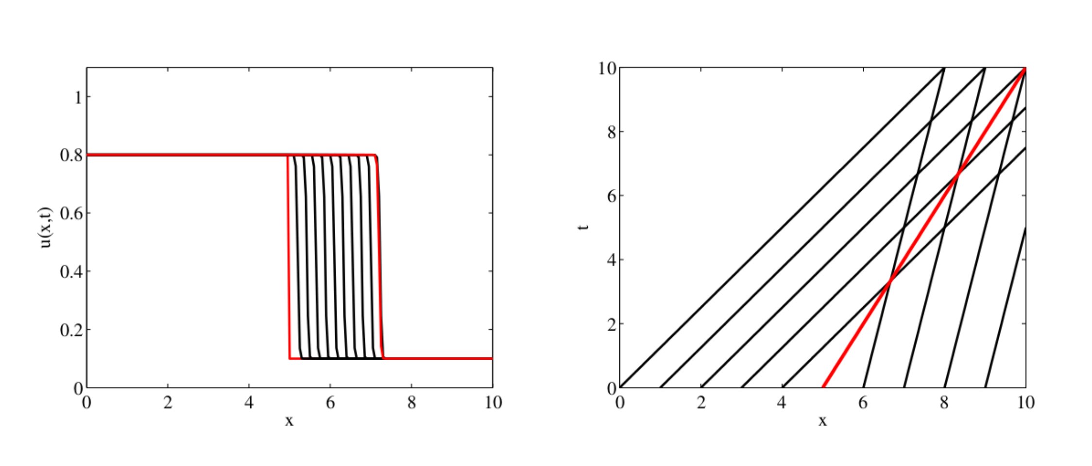
Riemann Problem with Burgers's equation

For the upwind case: \[ \begin{aligned} \frac{\partial u}{\partial t} + u \frac{\partial u}{\partial x }&= 0, \\ \text{with } u(x, 0)&= \begin{cases}u_L & x \leq 0 \\ u_R & x>0\end{cases} \end{aligned} \] with \(u_L>u_R\).

And the shock is created with a speed: \[ s = \frac{1}{2}(u_R+u_L) \] and the solution: \[ u(x,t) = \begin{cases} u_L & x \leq \frac{1}{2}t \\ u_R & x> \frac{1}{2}t\end{cases} \]

Example of non-unique reverse Riemann Problem with Burgers's equation

Reverse the initial condition in the previous example:

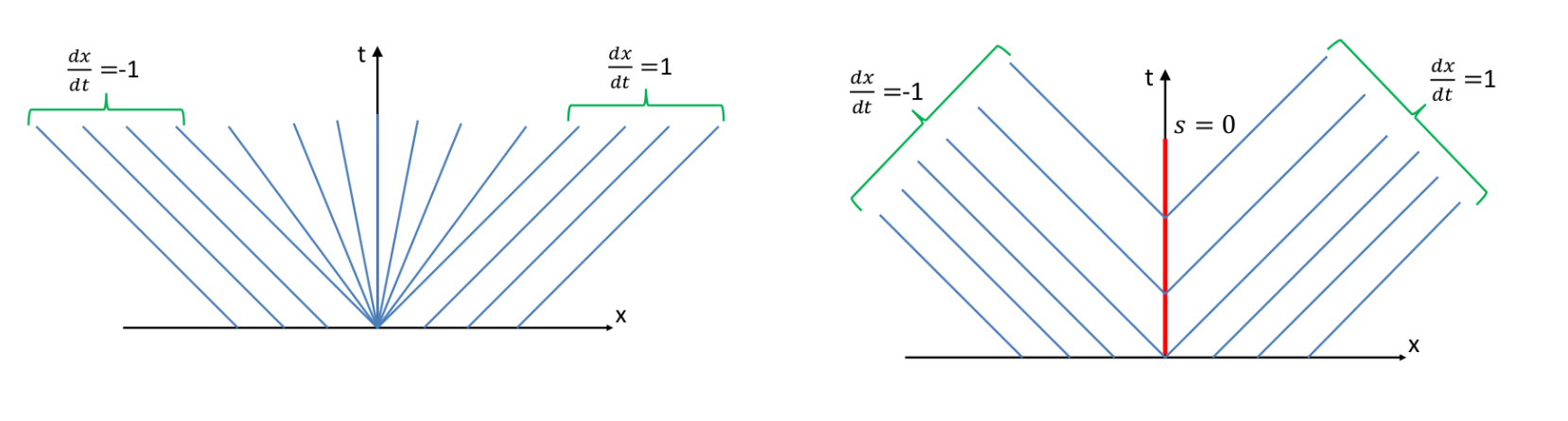
\[ \begin{aligned} \frac{\partial u}{\partial t} + u \frac{\partial u}{\partial x }&= 0, \\ \text{with } u(x, 0)&= \begin{cases}0 & x \leq 0 \\ 1 & x>0\end{cases} \end{aligned} \] the characteristics become:

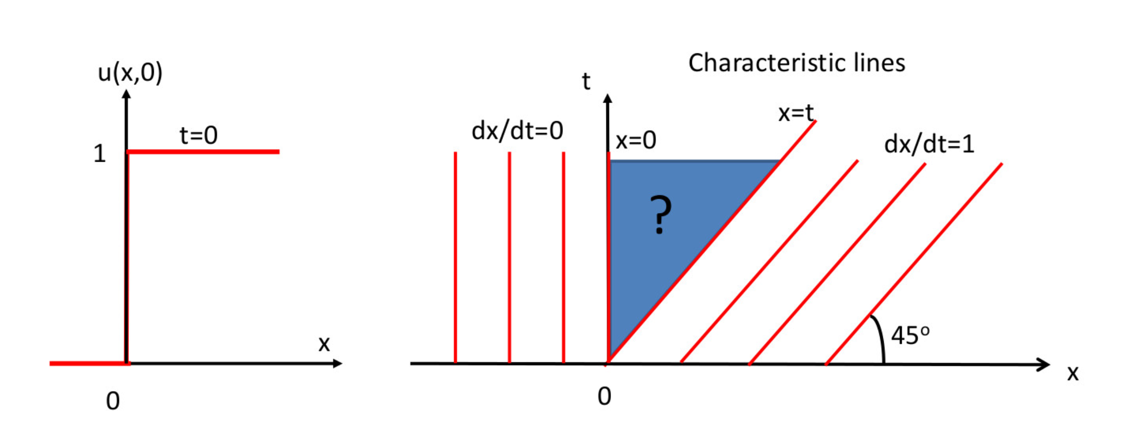
Solution in the blue area (\(0<x<t\)) is not defined. So here proposes 2 possible solutions, both are mathematical acceptable:

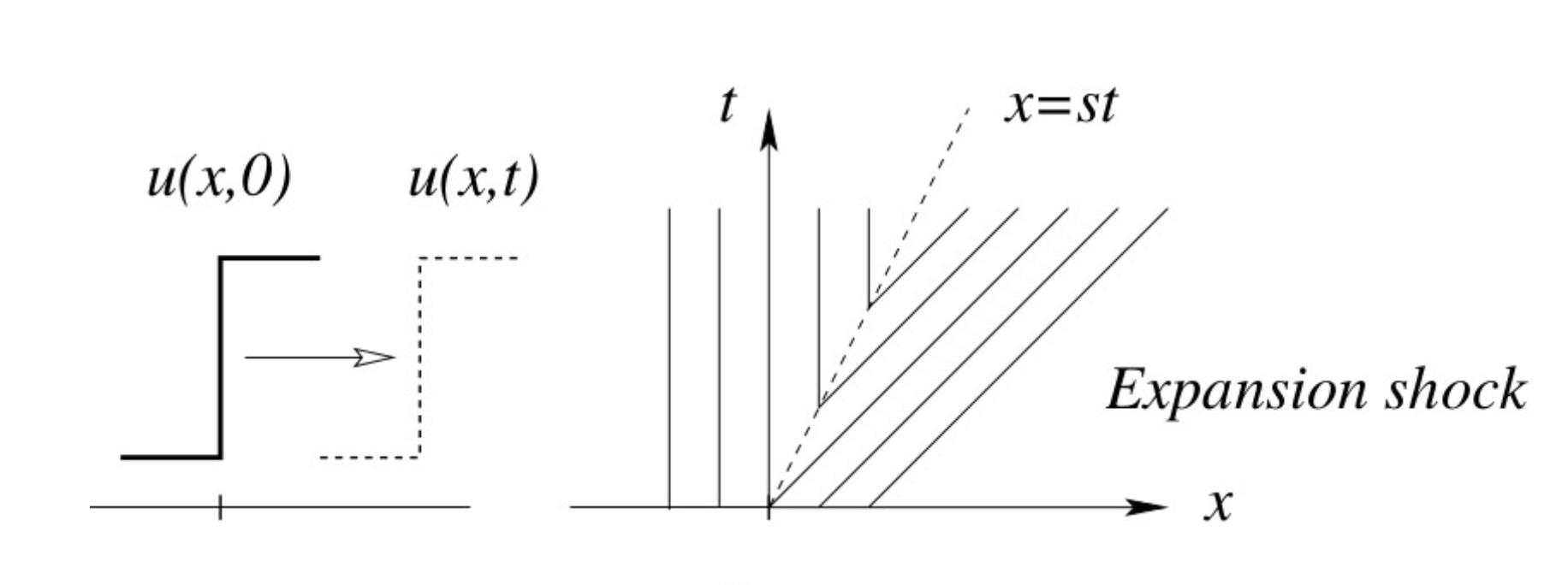
Solution A: \[ u(x, t)= \begin{cases}0 & \text { if } \quad \frac{x}{t}<s(=0.5) \\ 1 & \text { if } \quad \frac{x}{t}>s(=0.5)\end{cases} \]

Solution B: \[ u(x, t)=\left\{\begin{array}{ccc} 0 & \text { if } & \frac{x}{t}<0 \\ \frac{x}{t} & \text { if } & 0<\frac{x}{t}<1 \\ 1 & \text { if } & \frac{x}{t}>1 \end{array}\right. \]

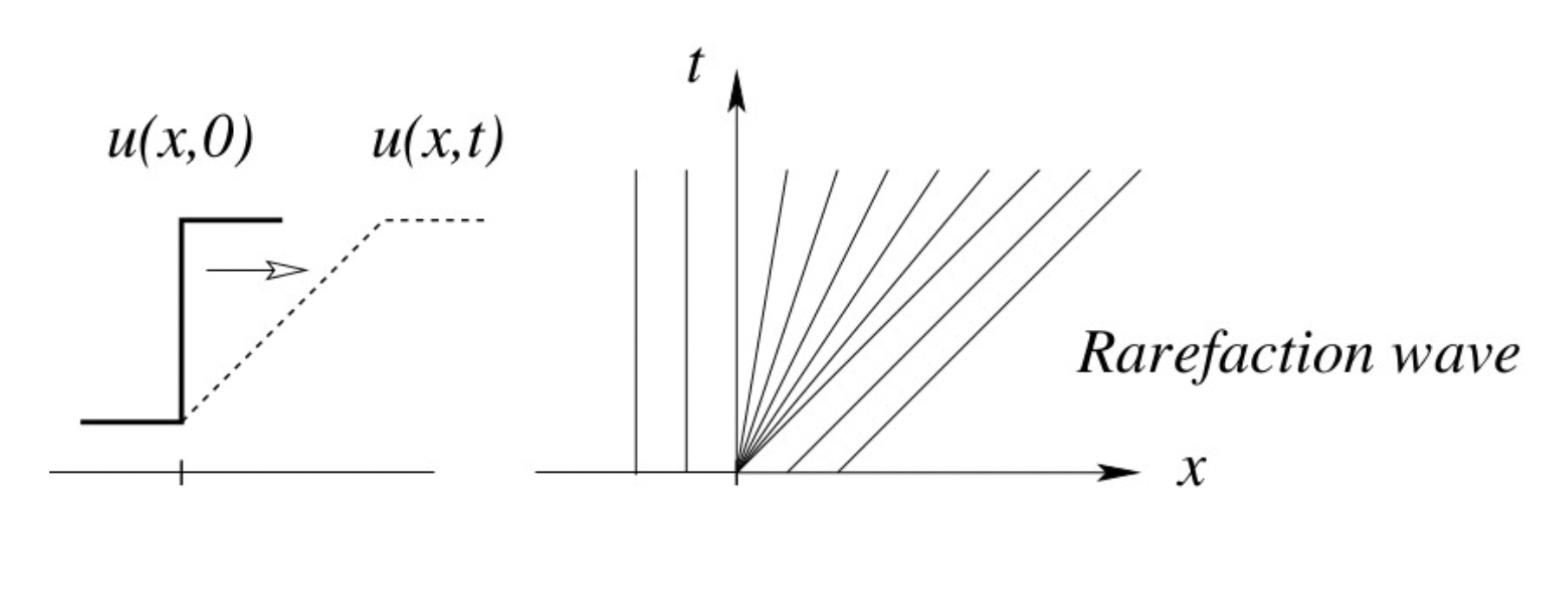
A little spoiler alert there: Solution B is physical, discussed in the next section.

Exact solution to Riemann Problem with Burgers's equation

In conclusion,

For the Riemann Problem with Burgers's equation: \[ \begin{aligned} \frac{\partial u}{\partial t} + u \frac{\partial u}{\partial x }&= 0, \\ \text{with } u(x, 0)&= \begin{cases}u_L & x \leq 0 \\ u_R & x>0\end{cases} \end{aligned} \]

• with \(u_L>u_R\)

  A shock wave is created with a speed: \[ V_s = \frac{u_L+u_R}{2} \] and the exact solution is: \[ u(x, t)=\left\{\begin{array}{ccc} u_L & \text { if } & \frac{x}{t}\leq V_s \\ u_R & \text { if } & \frac{x}{t}>V_s \end{array}\right. \]

• with \(u_L<u_R\)

  the exact solution is the rarefaction wave: \[ u(x, t)=\left\{\begin{array}{ccc} u_L & \text { if } & \frac{x}{t}<0 \\ \frac{x}{t} & \text { if } & 0<\frac{x}{t}<1 \\ u_R & \text { if } & \frac{x}{t}>1 \end{array}\right. \] if \(u_L = -u_R\), we have a sonic rarefaction wave.

Entropy Conditions

Why solution A is wrong? we need to impose additional conditions. There are two ways.

• Add a small diffusion term (2 ^nd order) manually on the RHS to remove the discontinuity. The weak solution then must satisfy: \[ \frac{\partial u^\epsilon}{\partial t} + \frac{\partial f(u^\epsilon)}{\partial x} = \epsilon\frac{\partial^2u^\epsilon}{\partial x^\epsilon} \] where \(\epsilon\) is the viscosity coefficient, it introduces the dissipation, known as the vanishing viscosity concept, into the equation to smooth the solution. A little bit cheating but most of people do this.

• Add the entropy solution

  I first hearted Entropy back in my undergraduate thermodynamic course. But I still don't know what is Entropy. So here are some answers:

  In gas dynamics, entropy is a constant physical quantity along particles in smooth flow which can jump to a higher value through a shock.

  The second law of thermodynamics says that entropy can never go down.

  For an evolution equation the information should always flow from the initial data.

  We can see it is very difficult to define it, but in order to translate the defination into the entropy condition, we see entropy as the extra amount of energy that is not available to the system.

  There are again two options of entropy condition:

  • Convex (concave) fluxes / Lax entropy condition \[ f'(u_L) > s > f'(u_R) \] and the characteristics must run into the shock, not emerge from it.

  • Oleinik entropy condition

    Similar to Lax entropy condition, it says: \[ \frac{f(u)-f(u_L)}{u-u_L}\geq s \geq \frac{f(u_R)-f(u)}{u_R-u} \]

  and Lax and Oleinik are equivalent if \(f(u)\) is strictly convex i.e. \(f''(u)<0\).

Numerical representation of discontinuities

Requirements on numerical schemes. Conservative discretisation: Lax-Wendroff theorem. First versus second order schemes. Representation of discontinuities: physical aspects, shock fitting/capturing.

Problems with Lax Equivalence Theorem

There are 3 fundamental properties of a numerical scheme:

• Consistency: how good you approximate operators and functions.

• Convergence: error between the exact and discrete solutions converges to zero.

• Stability: solution of the difference equation is not too sensitive to small perturbations.

The convergence needs to be evaluated with exact solutions. So we always need analytical solutions to verify it. If we don't have access to the analytical solutions, we have a Lax Equivalence Theorem says \[ \text{consistency + stability $\Rightarrow$ convergence} \] It is a fundamental convergence theorem but

• it is valid only for linear PDEs and there is no non-linear equivalent theorem
• this theorem does not tell if the weak solution physically acceptable or not.

For non-linear PDEs, we only have one experience,

If a scheme is stable on linear PDEs, it will often (not all the time) be stable on non-linear PDEs. If a scheme is unstable on linear, it won't be stable on non-linear.

So the work flow is, 1. Given a non-linear PDE, 2. Linearise it to explore the stabilities of schemes on it. 3. Test the winners on non-linear PDEs.

Schemes on linear advection equation

First we consider a 1D linear case, linear advection equation: \[ \frac{\partial u}{\partial t} + a\frac{\partial u}{\partial x} = 0 \] with \(a\) a positive scalar constant, representing the wave speed. So we have: \[ f(u) = au \]

Base finite difference scheme

try to solve it numerically, with finite difference, Euler forward difference in time and central difference in space. we have: \[ \frac{u^{n+1}_i-u^n_i}{\Delta t} + a \frac{u^n_{i+1}-u^n_{i-1}}{2\Delta x} = 0 \]

\[ u^{n+1}_i = u^n_i - \frac{a\Delta t}{\Delta x}\left(\frac{u^n_{i+1}-u^n_{i-1}}{2} \right) \]

It is consistency, and the Von Neumann analysis shows it is stable if the CFL condition (Courant number \(a\frac{\Delta t}{\Delta x}<1\)) is satisfied. It should converge to the exact solution.

Numerical practice

Consider a convection equation \[ \frac{\partial u}{\partial t} + \frac{\partial u}{\partial x} = 0 \] with a Riemann initial condition \[ u(x, 0)= \begin{cases} 1.2 &x \leq 0 \\ 0.4 & x>0\end{cases} \] The Euler in time, central difference in space scheme is applied on fortran script (base.f90, all the scripts in this post are annotated and modified from my graduate CFD course material). And the result is shown here:

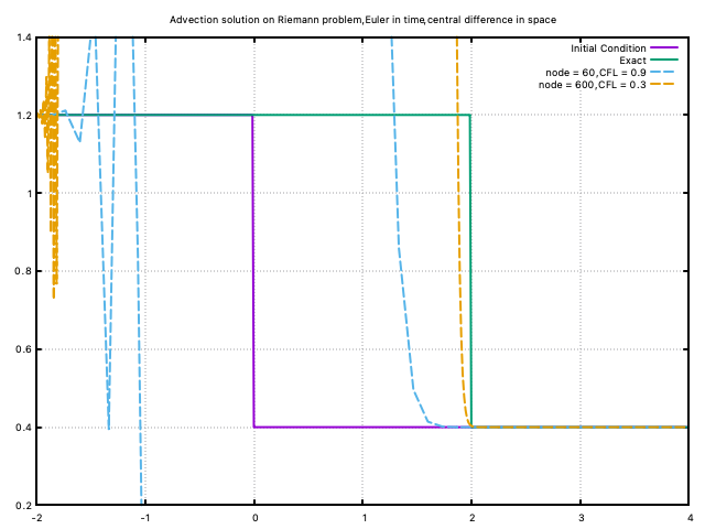
And the solver crashed, which means the scheme is unstable. And with finer mesh and smaller time step (controlled by Courant number), the scheme still does not converge to the exact solution.

Lax-Friedrich's scheme

Lax-Friedrich replaces the term \(u^n_i\) by the average \(u^n_i = \frac{1}{2}(u^n_{i+1}+u^n_{i-1})\), \[ u^{n+1}_i = \underbrace{\frac{u^n_{i+1}+u^n_{i-1}}{2}}_{\text{only change}} - \frac{a\Delta t}{\Delta x}\left(\frac{u^n_{i+1}-u^n_{i-1}}{2} \right) \]

Numerical practice

Based on the same equation and initial condition, with same time & space intervals, iteration times, Courant numbers, the Lax-Friedrich's scheme in time, central difference in space is applied (Lax-Friedrichs_scheme.f90). And the result is shown here:

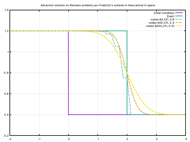
This scheme is a little better

• there are oscillations yet with smaller \(\Delta x\) and \(\Delta t\), the oscillations are smoothed out.
• the solution does not converge to the exact.
  • This scheme is highly diffusive and the discontinuity is more smoothed out with higher resolution.
  • The location of the shock is not captured.

1^st order Upwind method

Keep the Euler forward time difference, give up the order of the spatial central difference scheme to have a first order backward/forward scheme as: \[ \frac{\partial u}{\partial x}= \begin{cases} \frac{u^n_{i}-u^n_{i-1}}{\Delta x} &a \geq 0 \\ \frac{u^n_{i+1}-u^n_{i}}{\Delta x} & a<0 \end{cases} \] as a result: \[ u^{n+1}_i = \begin{cases} u^n_i - \frac{a\Delta t}{\Delta x}\left(u^n_{i}-u^n_{i-1} \right) &a \geq 0 \\ u^n_i - \frac{a\Delta t}{\Delta x}\left(u^n_{i+1}-u^n_{i} \right) & a<0 \end{cases} \]

The idea is that because the downstream of the shock will not feel the upstream, so this upwind scheme may be able to capture this kind of discontinuity.

Numerical practice

Similarly, Euler in time, First Order Upwind in space is applied on the same problem (first_order_upwind.f90. And the result is shown below:

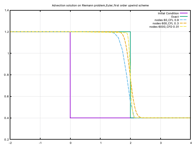
This scheme is the best so far,

• there is no oscillation because it is first order
• the solution converge to the exact
  • This scheme is slightly diffusive and the discontinuity is better captured with higher resolution.
  • The location of the shock is well captured.

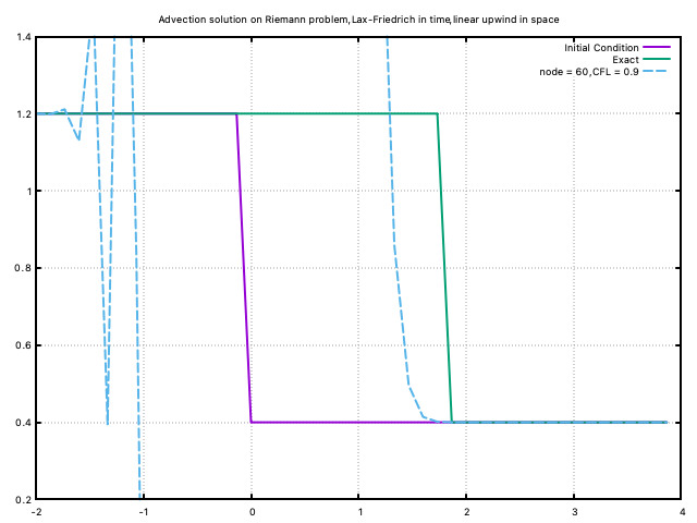
Just for fun, we can apply the Lax-Friedrich in time and first order upwind in space, we still have the oscillations. It is explainable, maybe because the Lax-Friedrich's scheme breaks the intent of the linear upwind scheme to isolate upwind information.

Lax-Wendroff scheme

It is one of the most well known second order schemes, based on the Taylor's theorem for \(u^{n+1}_i\): \[ u_{i}^{n+1} \approx u_{i}^{n}+\left.\Delta t \frac{\partial u}{\partial t}\right|_{i} ^{n}+\left.\frac{\Delta t^{2}}{2} \frac{\partial^{2} u}{\partial t^{2}}\right|_{i} ^{n}+\ldots \] with \(\frac{\partial u}{\partial t} = -a\frac{\partial u}{\partial x}\) and \(\frac{\partial u}{\partial t} = a^2\frac{\partial^2 u}{\partial x^2}\), plus the Euler scheme, we have: \[ u^{n+1}_i = u^n_i - \frac{a\Delta t}{\Delta x}\left(\frac{u^n_{i+1}-u^n_{i}}{2} \right) + \frac{a^2\Delta t^2}{\Delta x^2}\left(\frac{u^n_{i+1}-2u^n_{i}+u^n_{i-1}}{2} \right) \]

We know the original central space scheme creates the oscillations, and Lax-Wendroff decides to add an another second order derivative term. According to the NS equation, the second derivative acts like a viscous term, bringing the diffusion, so it might be able to stabilise the scheme.

This scheme is not consistent, because of this additional second order term.

Numerical practice

Euler in time, Lax-Wendroff scheme in space is applied on the same problem (Lax-Wendroff.f90). And the result is shown below:

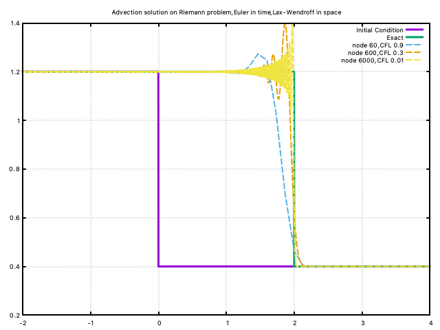
This scheme,

• the oscillation area on the top grows with the resolution
• the solution converge to the exact
  • The discontinuity is better captured with higher resolution.
  • The location of the shock is well captured.

The oscillated behaviour exist may be because the contribution of the stabiliser is too small. Try adding a coefficient to the second-order term, we have: \[u^{n+1}_i = u^n_i - \frac{a\Delta t}{\Delta x}\left(\frac{u^n_{i+1}-u^n_{i}}{2} \right) + \phi \frac{a^2\Delta t^2}{\Delta x^2}\left(\frac{u^n_{i+1}-2u^n_{i}+u^n_{i-1}}{2} \right)\] With code: Lax-Wendroff_coefficient.f90,

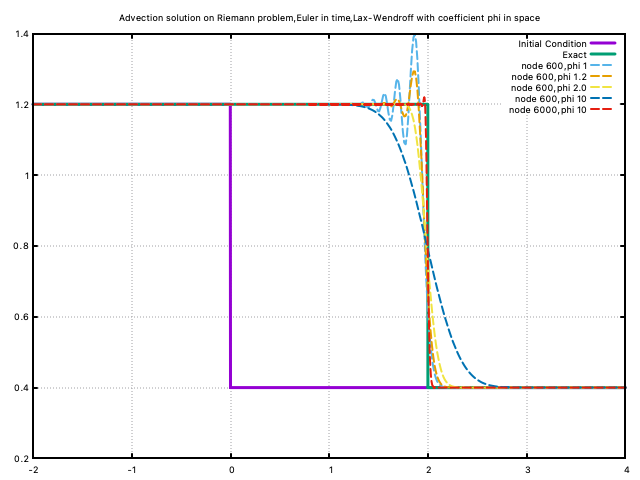
It can be seen that increasing the value of \(\phi\) brings more diffusion to the equation, and oppositely, increasing the number of nodes brings more oscillation to the system.

The appropriate value of \(\phi\) may be proportional to the mesh resolution. And actually it is also a function of the initial equation (the speed gap across the shock).

In conclusion,

• First order scheme is diffusive
• Second order scheme is dispensive
• First order solution is smooth / not accurate / stable (it is impossible for first order scheme to oscillate, it is the most used scheme in the industry when dealing with discontinuities)
• Second order solution is more accurate / oscillation (there is always more oscillations with more accurate solutions, more points, more values of the differences)

The goal is to balance the accuracy with oscillation.

Cancellation of oscillations is an active field of research

Schemes on non-linear Burger equation

After linear PDE, we consider a 1D non-linear case, burger equation, with two forms,

• primitive form: \[ \frac{\partial u}{\partial t} + u\frac{\partial u}{\partial x} = 0 \]

• conservative form: \[ \begin{aligned} \frac{\partial u}{\partial t} + \frac{\partial f(u)}{\partial x} = 0, \\ \text{with }f(u)=\frac{1}{2}u^2 \end{aligned} \]

1^st order upwind scheme

We consider forward difference (Euler) in time and 1^st order upwind (backward in this case) in space, we have

• primitive form: \[ \begin{aligned} \frac{\partial u}{\partial t} = \frac{u^{n+1}_{i}-u^{n}_{i}}{\Delta t} \\ \frac{\partial u}{\partial x} = \frac{u^{n+1}_{i}-u^{n}_{i}}{\Delta x} \end{aligned} \] As a result: \[ u^{n+1}_{i}= u^{n}_{i}-u^{n}_{i}\frac{\Delta t}{\Delta x}\left(u^{n+1}_{i}-u^{n}_{i}\right) \]

• conservative form: \[ \begin{aligned} \frac{\partial u}{\partial t} = \frac{u^{n+1}_{i}-u^{n}_{i}}{\Delta t} \\ \frac{\partial f(u)}{\partial x} = \frac{(u^{n+1}_{i})^2-(u^{n}_{i})^2}{2\Delta x} \end{aligned} \]

  As a result: \[ u^{n+1}_{i}= u^{n}_{i}-\frac{\Delta t}{2\Delta x}\left((u^{n+1}_{i})^2-(u^{n}_{i})^2\right) \]

Numerical practice

Consider a burger equation \[ \frac{\partial u}{\partial t} + u\frac{\partial u}{\partial x} = 0 \] with a Riemann initial condition \[ u(x, 0)= \begin{cases} 1.2 &x \leq 0 \\ 0.4 & x>0\end{cases} \] Euler in time, first order upwind (backward in this case)scheme in space is applied on the same Riemann problem(). Set endtime as 2.5 to maintain the same shock position as before. And the result is shown below:

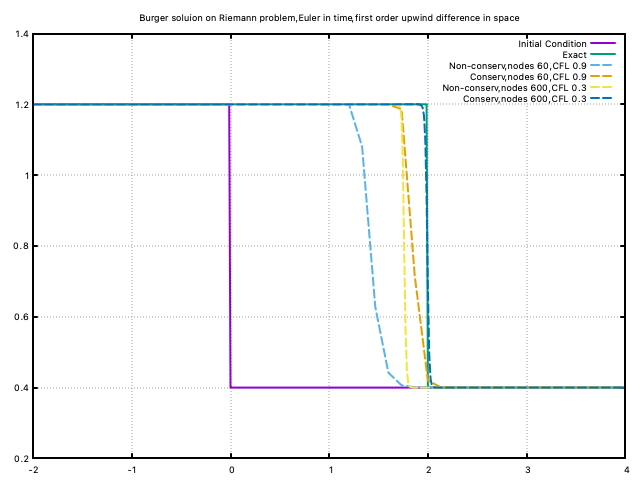
As we can see:

• the non-conservative form failed to locate the shock position properly.
• Increase the resolution, the conservative form converges nicely.

Conservative form performs better than the non-conservative, but the non-conservative form is alway easy to implement when dealing with the Euler equation. There is never a win-win situation.

Conservative Form Schemes

Now we know the conservative form is better, and here is a way of writing the scheme in the conservative form. First we need to go back the integral form with the finite volume methods.

Finite-Volume Methods

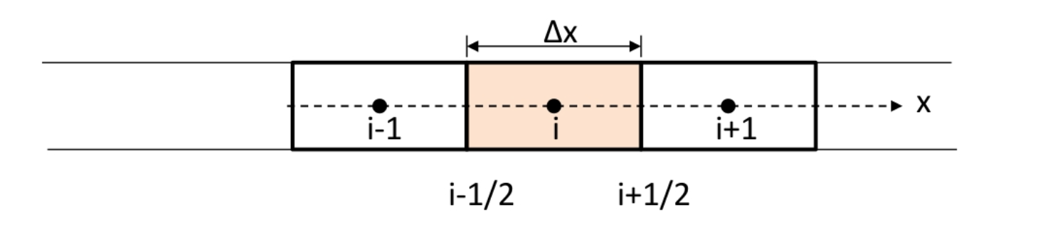
With the mesh above, we have the equation below, the change of cell values is only determined by the edge values. \[ \int_{x_{i-1 / 2}}^{x_{i+1 / 2}}\left[u\left(x, t^{n+1}\right)-u\left(x, t^{n}\right)\right] d x=-\int_{t^{n}}^{t^{n+1}}\left[f\left(u\left(x_{i+1 / 2}, t\right)-f\left(u\left(x_{i-1 / 2}, t\right)\right)\right] d t\right. \] Then define the cell-averaged \(\bar{u}_{i}^{n}\) and \(\bar{u}_{i}^{n+1}\) at time \(t^{n}\) and \(t^{n+1}\) : \[ \bar{u}_{i}^{n}=\frac{1}{\Delta x} \int_{x_{i-1 / 2}}^{x_{i+1 / 2}} u\left(x, t^{n}\right) d x \quad \bar{u}_{i}^{n+1}=\frac{1}{\Delta x} \int_{x_{i-1 / 2}}^{x_{i+1 / 2}} u\left(x, t^{n+1}\right) d x \] plus the time averaged flux \(f_{i-1 / 2}\) and \(f_{i+1 / 2}\) as \[ f_{i-1 / 2}=\frac{1}{\Delta t} \int_{t^{n}}^{t^{n+1}} f\left(u\left(x_{i-1 / 2}, t\right)\right) d t \quad f_{i+1 / 2}=\frac{1}{\Delta t} \int_{t^{n}}^{t^{n+1}} f\left(u\left(x_{i+1 / 2}, t\right)\right) d t \] We get the general form for a conservative numerical scheme: \[ \bar{u}_{i}^{n+1}=\bar{u}_{i}^{n}-\frac{\Delta t}{\Delta x} \left(f_{i+1 / 2}-f_{i-1 / 2}\right) \] We need consistency check as:

• for numerical flux \(f_{i+1 / 2}\): \(f\left(\ldots, \bar{u}_{i-1}, \bar{u}_{i}, \bar{u}_{i+1}, \ldots\right)=f(u)\)

• for the conservative scheme: the velocity can only change due to the fluxes:

  we can easily have: \[ (\bar{u}_{i-1}^{n+1}+\bar{u}_{i}^{n+1}+\bar{u}_{i+1}^{n+1})=(\bar{u}_{i}^{n-1}+\bar{u}_{i}^{n}+\bar{u}_{i}^{n+1})-\frac{\Delta t}{\Delta x} \left(f_{i+3 / 2}-f_{i-3 / 2}\right) \] passed.

Conservative Finite-Difference Methods

Inspired by the FVM methods, we have the general form of a conservative FDM method: \[ \color{purple} \bar{u}_{i}^{n+1}=\bar{u}_{i}^{n}-\frac{\Delta t}{\Delta x} \left(F^{n}_{i+1 / 2}-F^{n}_{i-1 / 2}\right) \] We can try to write the conservative version of most of the FDM methods, (but not all):

• Upwind method: \[ F^{n}_{i+1 / 2} = \frac{1}{2}(u^{n}_{i})^2 \]

• Lax-Friedrich's scheme: \[ F^{n}_{i+1 / 2} = \frac{\Delta x}{2\Delta t}(u^{n}_{i}-u^{n}_{i+1})+\frac{1}{2}\left[F(u^{n}_{i+1})+F(u^{n}_{i-1})\right] \]

Some facts about conservative methods:

• Conservative methods automatically locate the shocks correctly (only the location, not the shape)
• Conservative methods may show large spurious oscillation and smoothing near shocks
• If not strictly conservative, then incorrect shock speeds. One way to deal with is manually impose the Rankine-Hugoniot jump condition, with awareness of shock locations.

Two main strategies for discontinuities,

• shock capturing (99%)

  Use a numerical scheme, in general conservative and with some added mechanism, to ensure that an entropy solution is obtained. (what we will discuss next)

• shock fitting

  Shocks (and other discontinuities) are treated as internal boundaries and the jump conditions are imposed as compatibility conditions across them.

Moreover, here is a theorem which is not very influential:

Lax-Wendroff Theorem

If a consistent (numerical flux consistent with physical flux), conservative scheme for the numerical solution of a hyperbolic conservation law converges (as \(\Delta x \rightarrow 0\) and \(\Delta t\rightarrow 0\)), it converges to a weak solution.

• It's only a weak solution, not guarantee if it is physically acceptable
• not guarantee it actually does converge

Scheme on reverse Riemann problem

So far our schemes only meet the Riemann problems with \(u_L>u_R\), for the reverse problem, we consider the Burger equation with initial condition: \[ u(x,0)= \begin{cases} -1 &x<0 \\ 1 & x>0 \end{cases} \] We have two mathematical solutions as:

Numerical schemes

we set 2 different initial conditions:

\[ u_i^0= \begin{cases} -1 &i\leq0 \\ 1 & i>0 \end{cases} \]

\[ u_i^0= \begin{cases} -1 &i<0 \\ 0 &i=0 \\ 1 & i>0 \end{cases} \]

And use the first order upwind scheme as \[ \frac{\partial u}{\partial t}=\frac{u_i^{n+1}-u_i^{n}}{\Delta t}, \qquad \frac{\partial (1/2u^2)}{\partial x}= \begin{cases} \frac{(u_{i}^{n})^2-(u_{i-1}^{n})^2}{2\Delta x} &u_i^n\geq0 \\ \frac{(u_{i+1}^{n})^2-(u_i^{n})^2}{2\Delta x} & u_i^n<0 \end{cases} \]

Numerical Practice

Solving the system with reverse_burger_first_order_upwind.f90, we have the result:

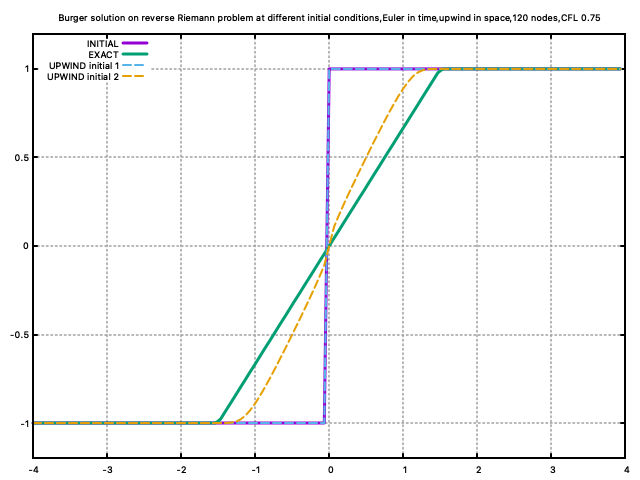
As we can see a single change of the initial condition results in different solutions.

• conservative methods can converge to non-physical solutions rather than to the physically correct rarefaction wave.
• the solution is very sensitive to initial data.

Actually it is also very sensitive the node number, and the CFL number, we change the nodes number to 100, keep the initial condition that converges to the entropy satisfying solution, we have another weak solution.

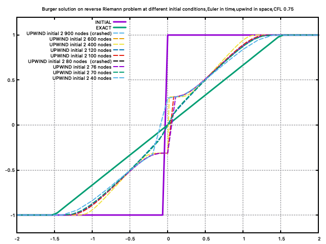
Different node number i.e. mesh resolution result in different weak solutions. Two main findings:

• The code crashed at some node numbers.
• Two types of solutions are found, either almost align with the smooth former result, or presents a bumpy at the centre.
• The relationship between the node number and the type of the solutions possesses a bifurcation behaviours.

I can't explain... Maybe still because the initial condition slightly changes with different resolutions. Need more work on searching more nodes numbers, and more initial condition settings.