Review of Physical Informed Neural Network

It's a brief note of the review paper: Physics-informed machine learning^[1] by the same group proposing the PINN^[2], including Prof. George Em Karniadakis and Dr. Lu Lu. Basic concepts and typical applications are introduced, as well as limitations and future directions.

Additional resources:

Papers:

• Physics-informed machine learning. Karniadakis, G. E., Kevrekidis, I. G., Lu, L., Perdikaris, P., Wang, S., & Yang, L. (2021).

• Physics-informed neural networks: A deep learning framework for solving forward and inverse problems involving nonlinear partial differential equations. Raissi, M., Perdikaris, P., & Karniadakis, G. E. (2019)

• Physics Informed Deep Learning (Part I): Data-driven Solutions of Nonlinear Partial Differential Equations, M.Raissi, P.Perdikaris, G.E.Karniadakis

• Physics Informed Deep Learning (Part II): Data-driven Discovery of Nonlinear Partial Differential Equations, M.Raissi, P.Perdikaris, G.E.Karniadakis

Course and slides:

• CS 598: Deep Generative and Dynamical Models
• CS598: Physics-Informed Neural Networks: A deep learning framework for solving forward and inverse problems involving nonlinear PDEs
• 20211210_pinn/pinn.pdf
• Physics-Informed Neural Networks (PINNs)

Blog and talk:

• Physics Informed Deep Learning
• DS1 Physics Informed Neural Networks
• Physics-Informed Deep learning(物理信息深度学习）
• Hidden Fluid Mechanics
• Hidden Physics Models AFMS Webinar 2021 #9 - Dr Maziar Raissi (University of Colorado)

Notes by sections

0. Abstract

Despite the strength of traditional simulation methods, (FVM and FEM ...), the weakness still exist such as:

• Troublesome to deal with complex problems:
  • mesh generation on complex boundary
  • curse of dimensionality, high-dimensional problem
• Nearly impossible to exploit observations:
  • incorporate available data (always noisy) seamlessly
  • solve inverse problem*

Obviously machine learning is designed to solve inverse problems with high dimensional data. Only problems are

• the requirement of big input data
• low interpretation

Physics informed learning integrating these methods.

The most attractive advantage is the ability to impose seamlessly physical law(constrains) on general machine learning model. With these constrains, the physical informed neural network will converge with much less data. And the interpretation can be improved as well.

*Inverse problem: solving a problem from observations with part of knowledge of the mathematical model i.e. PDE.

PINN still not belongs to fully Interpretable Neural Networks. Yet there is always a trade-off between interpretation and good performance.

	FEM/FVM/FDM	PINNS	ROMs*
Solution Space	Basis Functions	Neural Networks	Smart Basis Functions
Differential Operators	Discretization/Weak-form	Automatic Differentiation	Discretization/Weak-form
Solver	Linear/non-linear/Iterative	Gradient Descent (Training)	Linear/non-linear/Iterative
Evaluate	Interpolation	Inference	Interpolation

ROMs: reduce order models, a generalisation of FEM/FVM/FDM the basis functions are carefully chosen based on previous timeSteps, similar geometries, or experience.

Same thing can be done on NNs, and it is the method of transfer learning. Pre-train models on carefully chosen problems. Then use the parameters to warm-start the training of NNs on another type of physics or geometries.

1. Introduction

Key idea

The key points are learning from

• Dinky, Dirty, Dynamic, Deceptive data and
• Scientific domain knowledge
  • e.g. physical principles, constrains, symmetries, computational simulations

to develop a model that is:

• Accurate, Robust, Reliable, Interpretable, Explainable

Instead of learning from the scratch, the developed valuable knowledge should also be exploited.

prior knowledge stemming from our observational, empirical, physical or mathematical understanding of the world can be leveraged to improve the performance of a learning algorithm

Data and Physics

There are 3 scenarios when solving physical problems shown below:

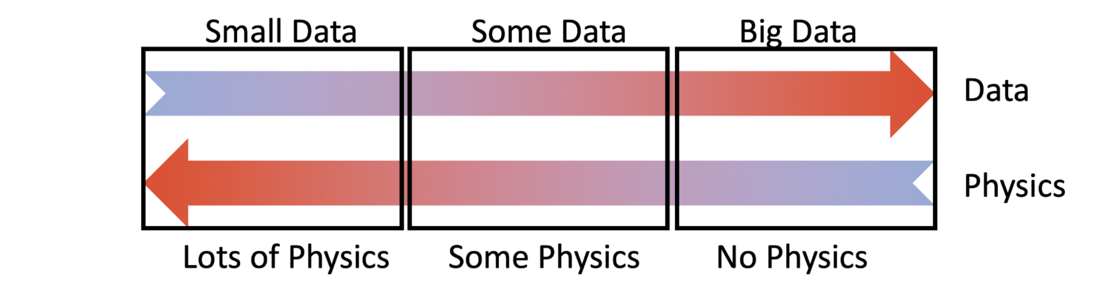
Forward problem	Inverse problem	System identification
Physics based (complete PDE)	Some physics (PDE, apart from BC, Initial, constants, params...)	Physics free
Data free	Small/noisy data	Data based
FDM, FEM, FVM	Multi-fidelity learning PINN DeepM&Mnet	NN Operator learning (DeepONet)

Inverse problem is also called data assimilation problem

System identification is also called model discovery

The paper focus mostly on the last 2 scenarios and a lot of prior works are listed:

Prior works

2. Method

How to embed physics in ML

There are 3 methods of imposing constrains into Neural Networks

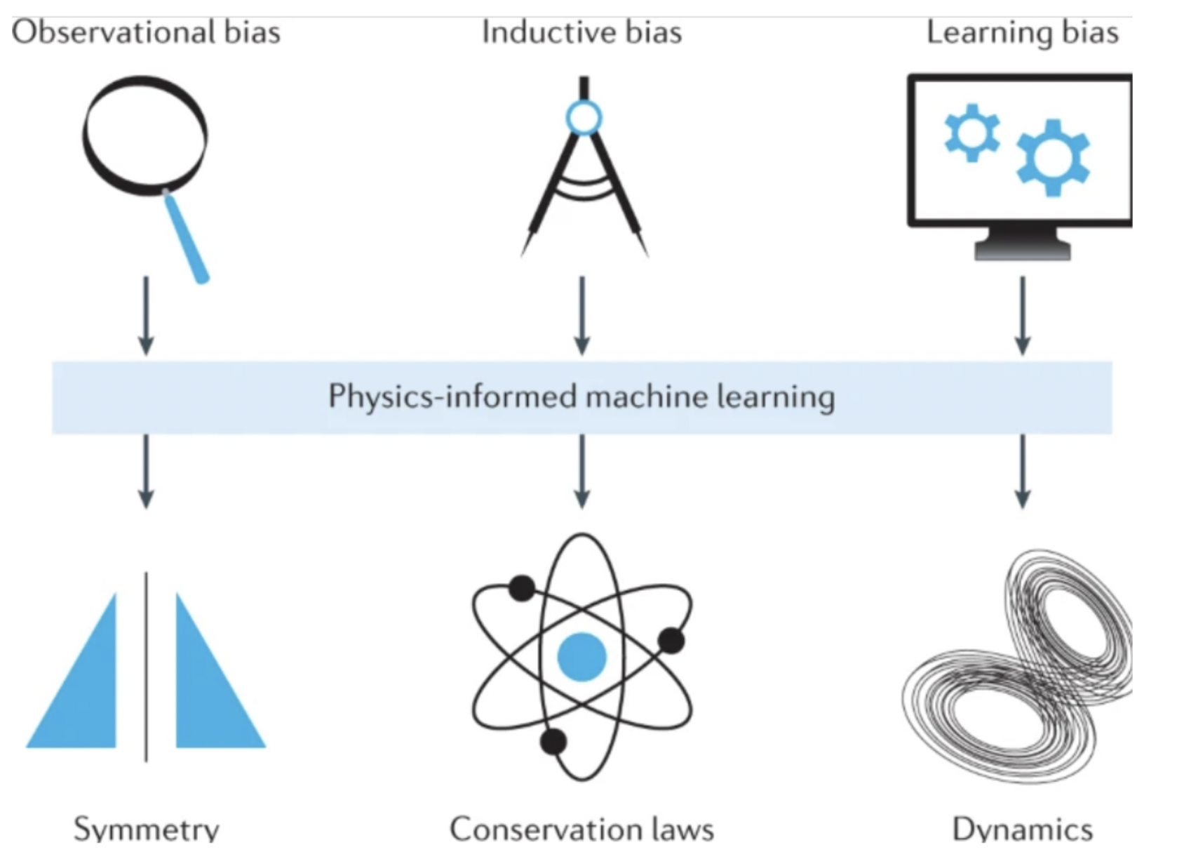
Observational biases

Directly from data, same as general NN methods, there are examples such as refs^{[16][17][18] [19]}.

Techniques such as data augmentation can be useful. e.g., if some bias such as symmetry is known, symmetric data augmentation a good choice.

Yet

• Difficult to find the symmetry and invariances.
• need big amount of data, which will cost a lot in most of the industrial areas.

Inductive biases

Embed the prior knowledge into architectures.

e.g.

• CNNs possess translation invariance because of the "convolution" algorithm.

• Dirichlet BC below can be embedded such as:

  \[ \text{BC:} \qquad u(0)=0, u(1)=1 \]

  \[ \begin{aligned} g(x)=x, \ell(x)=x(1-x) \\ \mathcal{N}(x)=g(x), \quad x \in \Gamma_D \subset \Omega \\ \hat{u}(x)=g(x)+\ell(x) \mathcal{N}(x) \\ \begin{cases}\ell(\mathbf{x})=0, & \mathbf{x} \in \Gamma_D \\ \ell(\mathbf{x})>0, & \mathbf{x} \in \Omega-\Gamma_D\end{cases} \end{aligned} \]

  a carefully designed activation function is added after the last layer so that the output satisfies such conditions.

• For periodic boundary conditions, take the idea of Fourier series, add a Fourier layer after the input as shown:

  

• For divergence-free system, \[ \nabla\cdot\mathbf{f} = 0 \] With the knowledge of \[ \text{divergence of the curl is 0: } \quad \nabla\cdot (\nabla\times g) \equiv 0 \] choose: \[ \mathbf{f} = \nabla \times g \]

  a \(curl\) function is added after the last layer so that the result is unconditionally divergence-free.

It is nearly free, automatically and exactly.

• do it if possible
• designed case by case
• limited to relatively simple and well-posed physics
  • require craftsmanship and elaborate implementations
  • extension to more complex tasks is challenging

Learning biases

This is the most general method, the idea is

• tinkering/penalising the loss function
• modulate the training process

Several examples include deep galerkin method^[22], PINN and its extensions^[23][24][25]. And PINN is mainly discussed.

PINN is a highly flexible framework that allows one to incorporate more general instantiations of domain-specific knowledge into ML models. Besides, the backend NN can be changed into CNN and RNN.

PINN method

Example

The method and paradigm of PINN can be illustrated via a typical example of solving a inverse problem: invisible cloaking design^[26].

PINN is compatible with not only inverse problems, forward problems, operator learning are also in its scope. See DeepXDE demos.

The title looks daunting but the problem is simple, relatively.

As shown above, a constant electrical field \(E_1\) will be perturbed by a metal cylinder inside with a permittivity \(\epsilon_3\). But this perturbation can be zero out by warping the cylinder with an extra "coat" with permittivity \(\epsilon_2\).

Goal:

Given \(\epsilon_1, \epsilon_3\), solve \(\epsilon_2(x,y)\) s.t. \(E_1 = {E_{1}}_{org}\)

Physical system:

Helmholtz equation \(\left(k_0=\frac{2 \pi}{\lambda_0}\right)\) \[ \nabla^2 E_i+\epsilon_i k_0^2 E_i=0, \quad i=1,2,3 \] Boundary conditions:

• Outer circle: \(E_1=E_2, \frac{1}{\mu_1} \frac{\partial E_1}{\partial \mathbf{n}}=\frac{1}{\mu_2} \frac{\partial E_2}{\partial \mathbf{n}}\)
• Inner circle: \(E_2=E_3, \frac{1}{\mu_2} \frac{\partial E_2}{\partial \mathrm{n}}=\frac{1}{\mu_3} \frac{\partial E_3}{\partial \mathrm{n}}\)

PINN architecture:

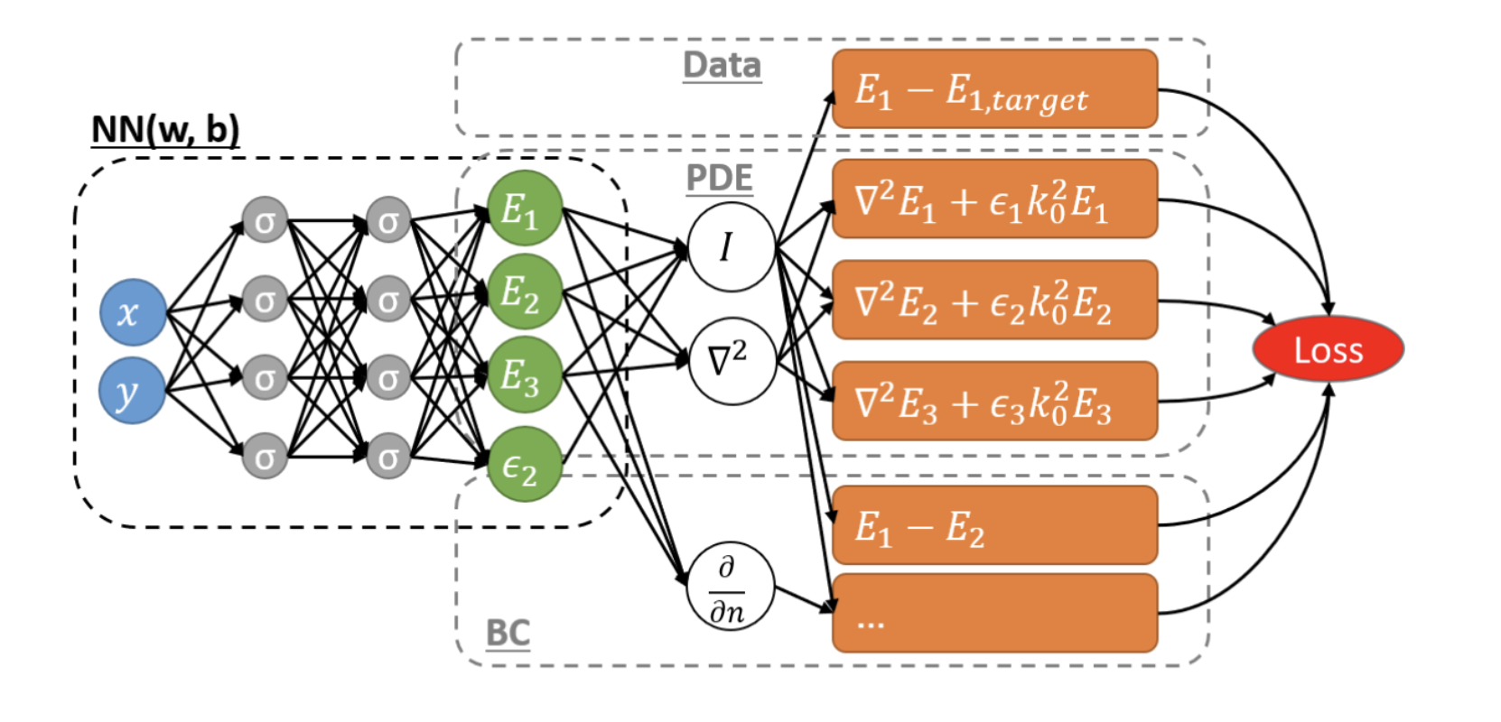
We can design a PDE embedded MLP as

• input: \(x, y\)
• output: \(E1,E2,E3,\epsilon_2\)
• loss function: blended function with observation loss and physical loss

note that in PINN, the derivatives (e.g. \(\nabla\) here) is calculated analytically by auto differentiation, no discretisation is needed, i.e. mesh-free & particle free.

In PINN, higher order auto differentiation could be needed in forward and back propagation (1 higher order than forward). In general NN, only 1^st order derivative is calculated in the process of back propagation.

Theory

PINN: \[ f\left(\mathbf{x} ; \frac{\partial u}{\partial x_1}, \ldots, \frac{\partial u}{\partial x_d} ; \frac{\partial^2 u}{\partial x_1 \partial x_1}, \ldots, \frac{\partial^2 u}{\partial x_1 \partial x_d} ; \ldots ; \boldsymbol{\lambda}\right)=0, \quad \mathbf{x} \in \Omega \]

• Initial/boundary conditions \(\mathcal{B}(u, \mathbf{x})=0\) on \(\partial \Omega\)

• Extra information \(\mathcal{I}(u, \mathbf{x})=0\) for \(\mathbf{x} \in \mathcal{T}_i\)

\[ \min _{\boldsymbol{\theta}, \boldsymbol{\lambda}} \mathcal{L}(\boldsymbol{\theta}, \boldsymbol{\lambda} ; \mathcal{T})=w_f \mathcal{L}_f\left(\boldsymbol{\theta}, \boldsymbol{\lambda} ; \mathcal{T}_f\right)+w_b \mathcal{L}_b\left(\boldsymbol{\theta}, \boldsymbol{\lambda} ; \mathcal{T}_b\right)+w_i \mathcal{L}_i\left(\boldsymbol{\theta}, \boldsymbol{\lambda} ; \mathcal{T}_i\right) \] where \[ \begin{aligned} \mathcal{L}_f &=\frac{1}{\left|\mathcal{T}_f\right|} \sum_{\mathbf{x} \in \mathcal{T}_f}\left\|f\left(\mathbf{x} ; \frac{\partial \hat{u}}{\partial x_1}, \ldots ; \frac{\partial^2 \hat{u}}{\partial x_1 \partial x_1}, \ldots ; \boldsymbol{\lambda}\right)\right\|_2^2 \\ \mathcal{L}_b &=\frac{1}{\left|\mathcal{T}_b\right|} \sum_{\mathbf{x} \in \mathcal{T}_b}\|\mathcal{B}(\hat{u}, \mathbf{x})\|_2^2 \\ \mathcal{L}_i &=\frac{1}{\left|\mathcal{T}_i\right|} \sum_{\mathbf{x} \in \mathcal{T}_i}\|\mathcal{I}(\hat{u}, \mathbf{x})\|_2^2 \end{aligned} \]

Not surprisingly, the blending factors \(w_f, w_b, w_i\) needed to be tuned.

Error analysis

This section needs extra care. In my understanding, it says the classic theory says NN is dense only in first order, which is sufficient for general NN, not for PINN.

Theorem (Universal approximation theorem; Cybenko, 1989)^[31] Let \(\sigma\) be any continuous sigmoidal function. Then finite sums of the form \(G(x)=\sum_{j=1}^N \alpha_j \sigma\left(w_j \cdot x+b_j\right)\) are dense in \(C\left(I_d\right)\).

universal approximators: standard multilayer feedforward networks are capable of approximating any measurable function to any desired degree of accuracy

Yet this theory has been extended to any higher order, which supports PINN well.

Theorem (Pinkus, 1999)^[32] Let \(\mathbf{m}^i \in \mathbb{Z}_{+}^d, i=1, \ldots, s\), and set \(m=\max _{i=1, \ldots, s}\left(m_1^i+\cdots+m_d^i\right)\). Assume \(\sigma \in C^m(\mathbb{R})\) and \(\sigma\) is not a polynomial. Then the space of single hidden layer neural nets \[\mathcal{M}(\sigma):=\operatorname{span}\left\{\sigma(\mathbf{w} \cdot \mathbf{x}+b): \mathbf{w} \in \mathbb{R}^d, b \in \mathbb{R}\right\}\] is dense in \[C^{\mathbf{m}^1, \ldots, \mathbf{m}^s}\left(\mathbb{R}^d\right):=\cap_{i=1}^s C^{\mathbf{m}^i}\left(\mathbb{R}^d\right)\]

Optimisation & Generalisation analysis can read Shin et al., 2020; Mishra & Molinaro, 2020; Luo & Yang, 2020

3. Merits of PINN

Problem related merits:

Flexible:

• Support different NN backends: MLP, CNN, RNN, GNN, GAN, Transformer etc...

• Support different disciplines: conservation laws, stochastic and fractional PDEs.

Different problems

• effective on ill-posed inverse problem
• not effective on well-posed, no data needed forward problem

Tackling high dimensionality

• unlike FVM/FDM or particles method, PINN is mesh free. So high dimensionality is not a problem.
• used to solve high-dimensional Black–Scholes, Hamilton–Jacobi–Bellman and Allen–Cahn equations^[30]

Strong generalisation in small data regime

Simple to implement in parallel

Additional merits:

• Help understand deep learning
  • provide theoretical insight and elucidate the inner mechanisms behind the surprising effectiveness of deep learning.
• Uncertainty quantification
  • uncertainties include the physics, data, and learning models
    • stochastic physical systems
      • described by stochastic PDEs/ODEs
      • GANs performs well on solving stochastic PDEs in high dimensions
    • data: aleatoric uncertainty arising from the noise in data and epistemic uncertainty arising from the gaps in data
      • Gaussian process regression (GPR) based PINN quantify uncertainty naturally, see ref^[27] and its talk. Yet the scalability is low. (For NN, mini batch SGD can deal with big data.)
      • An extension B-PINNs^[29] can provide reasonable uncertainty bounds

!Not fully understand, need knowledge of stochastic systems.

So far I see data uncertainty quantification as a way of controlling overfitting and underfitting, i.e. bias and variance. (Recall underfitting - low bias and high variance, overfitting - high bias and low variance)

Uncertainty in NNs can be partly quantified by techniques such as dropout, regularisation.

4. Applications

Only fluid related works is presented here, more in the paper.

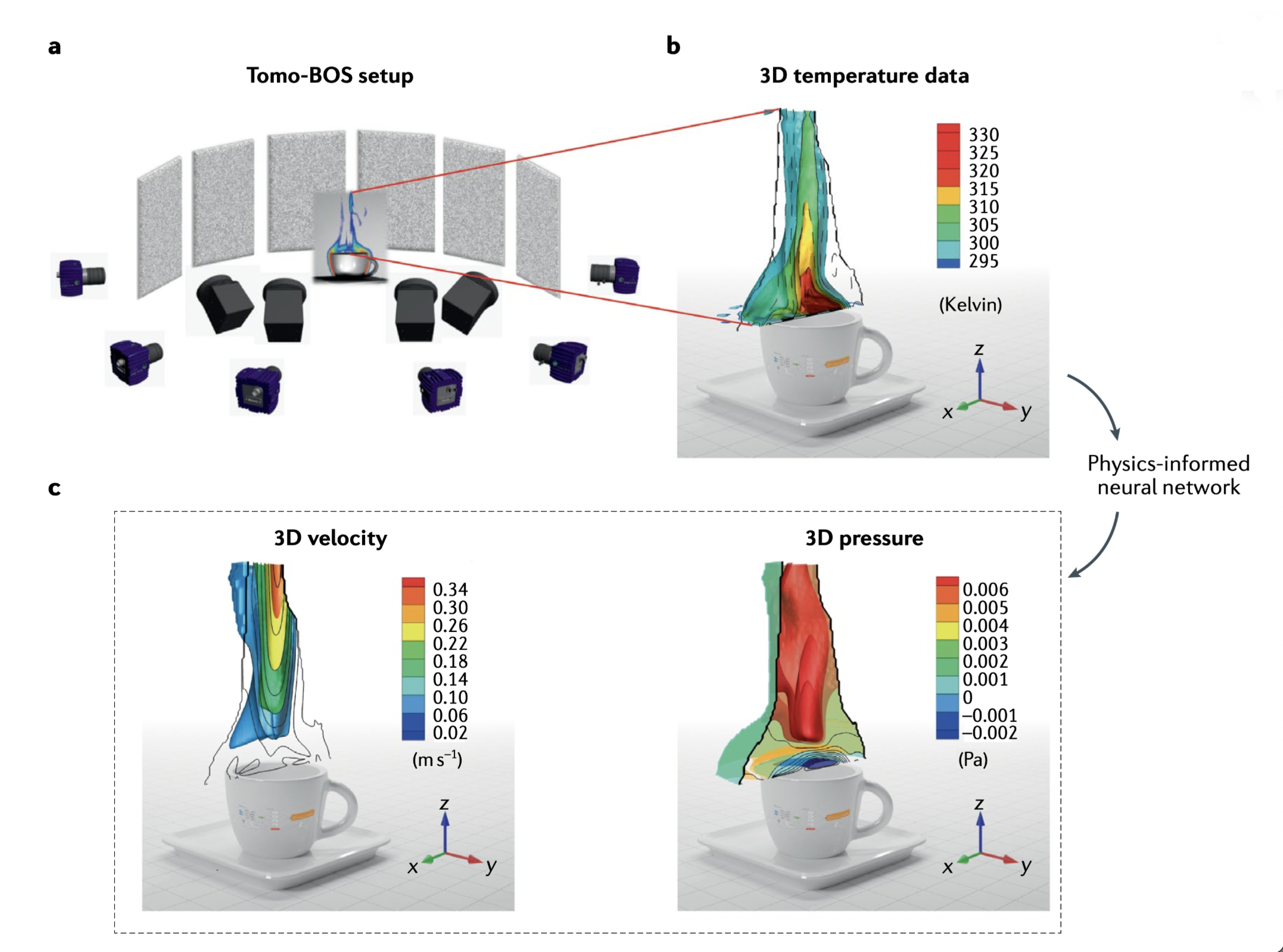
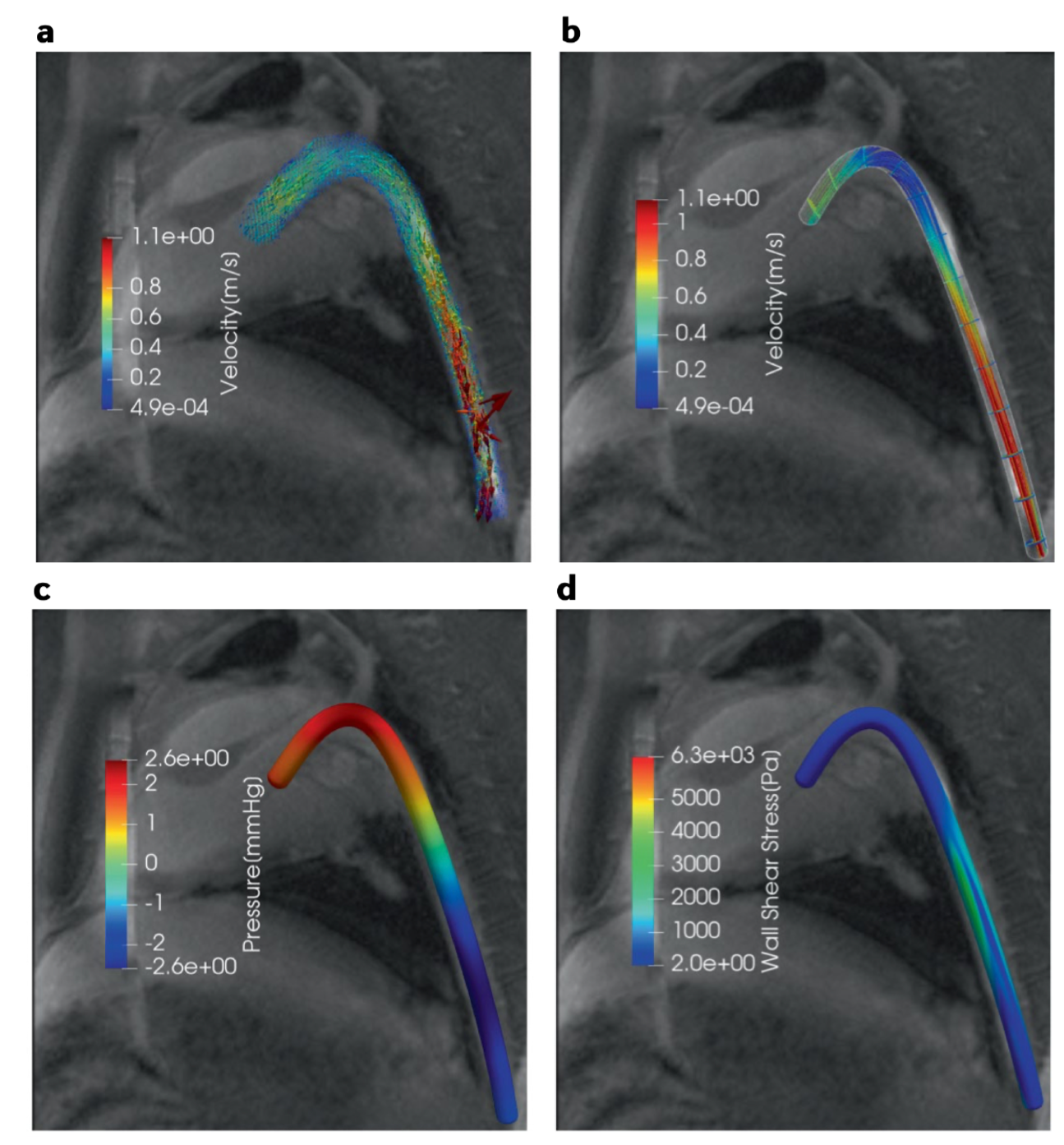
Field inferring^[33]

The pressure and velocity can be inferred based on the temperature field. We know the N-S function, but the viscosity, boundary are not known.

Field denoising^[34]

Similarly, if the input data is scattered and noisy, PINN is a method to construct the fluid field with a smooth and boundary-clear result. Other important fields (biomarkers) can be inferred seamlessly.

5. Limitations

These limitations are also the treading research areas:

Complex systems

• High-frequency components of multiscale systems
  • high frequency is too much for MLP, the most common base of PINN
    • extra tricks is needed
• computational complex on multiphysics system
  • ref^[3] based on DeepM&M is a good example to deal with it
• loss function fail on specific problems
  • traditional point-wise will fail on
    • high-dimensional problems
    • some special low-dimensional cases

New algorithms and computational frameworks

• non-convex optimisation problems

  • inherited from the Neural Networks
  • global minim cannot be guaranteed
  • refs^[4][5][6] discuss more of it

• time consuming on tuning

  • inherited from the Neural Networks
  • autoML^[7] techniques are emerging to solve this problem
  • architecture teaching^[8], meta-learning^[9] etc

• transfer leaning

  • popular idea in ML world
  • ref^[10] is a good attempting

• efficient higher order derivatives algorithms

  • specific need for PINN, in general NN, only 1st order derivative is needed

  • not well supported by mainstream ML frameworks (tf and torch)

  • Taylor-mode automatic differentiation provides better support

Database and benchmark supports

• UCI Machine Learning Repository^[11]
  • noise generated by an aerofoil
  • ocean temperature and current measurements related to El Niño
  • hydrodynamic resistance related to different yacht designs
• data is not available in many different applications
• standard benchmarks needed

More mathematical understanding

• improve the understanding on NN and PINN
• improve the interpretation
• potential to
  • more robust and effective training algorithms,
  • build a solid foundation for NN and PINN

6. Outlooks

Visualisation tool, need more of general TensorBoard, requirement to visualise the field solution on the fly, just like OpenFOAM.

Potential of digital twins, several problems are pointed out:

• complexity of observations data: noisy, scarce, multi-modility
• need time consuming pre-processing and calibrations
• the control function always need extra constitutive laws to close

Importance of building ML-based transformations between predictive models

The normal paradigm need choose humanly interpretable observables/variables and a ‘reasonable’ dictionary of operators based on the chosen observables. Possibility to automatically determine variables physical model formulations.

Active learning - data collection while training, determine what data to collect and what formulation to choose actively.

Ultimately change the way of thinking.

PINN family

PINN has been a hit in science and math fields since its publish. Several following works are also published afterwards. Here are some of them:

B-PINN^[35]

As mentioned before, unlike the Bayesian framework (e.g. GP), NN cannot provide uncertainty bounds. B-PINN integrate the Bayesian approach with PINN. When it comes to ill-posed problems and imperfect data, B-PINN is suitable. Yet prior for B-PINNs in a systematic way is still an open question.

HPINN^[36]

Physics-informed neural networks with hard constraints (hPINNs). Recall the loss function of PINN, it is a blended function and each term cannot be perfectly satisfied (soft constraints). The Augmented Lagrangian method is used together with the loss function to make sure a hard constraints on the control function.

FPINN^[37]

Origin PINN are suitable for integer-order partial differential equations (PDEs). FPINN extend the functions to Fractional Differential Equations.

gPINN with RAR^[38]

Residual-based adaptive refinement (RAR^[39]). Uniform residual points are not efficient for PDEs with steep solutions. RAR adaptively add more points in locations with large PDE residual.

Gradient-enhanced PINN. Taking the idea that the derivatives of the PDE residual are also zero. gPINN embeds the gradient of the PDE residual into the loss.

CPINN^[40] and XPINN^[41]

Conservative physics-informed neural networks on discrete domains for conservation laws. The computational domain is decomposed and flux continuity is imposed in the strong form along the sub-domain interfaces. Enable PINN of parallelisation.

eXtended PINNs: A generalised space-time domain decomposition based deep learning framework. Extend the conservation laws of CPINN to any type of PDEs. And the domain can be decomposed in any arbitrary way (in space and time, space and time parallelisation). Larger representation and parallelisation capacity, effective for multi-scale and multi-physics problems.

References

1. Karniadakis, G. E., Kevrekidis, I. G., Lu, L., Perdikaris, P., Wang, S., & Yang, L. (2021). Physics-informed machine learning. Nature Reviews Physics, 3(6), 422-440. ↩︎
2. Raissi, M., Perdikaris, P., & Karniadakis, G. E. (2019). Physics-informed neural networks: A deep learning framework for solving forward and inverse problems involving nonlinear partial differential equations. Journal of Computational physics, 378, 686-707. ↩︎
3. Cai, S., Wang, Z., Lu, L., Zaki, T . A. & Karniadakis, G. E. DeepM&Mnet: inferring the electroconvection multiphysics fields based on operator approximation by neural networks. J. Comput. Phys. 436, 110296 (2020). ↩︎
4. Wang, S., Yu, X. & Perdikaris, P . When and why PINNs fail to train: a neural tangent kernel perspective. Preprint at arXiv https://arxiv.org/abs/2007.14527 (2020). ↩︎
5. Wang, S., Wang, H. & Perdikaris, P . On the eigenvector bias of Fourier feature networks: from regression to solving multi-scale PDEs with physics-informed neural networks. Preprint at arXiv https://arxiv.org/abs/ 2012.10047 (2020). ↩︎
6. Wang, S., T eng, Y. & Perdikaris, P . Understanding and mitigating gradient pathologies in physics- informed neural networks. Preprint at arXiv https://arxiv.org/ abs/2001.04536 (2020) ↩︎
7. He, X., Zhao, K. & Chu, X. AutoML: a survey of the state- of-the- art. Knowl. Based Syst. 212, 106622 (2021). ↩︎
8. Elsken, T ., Metzen, J. H. & Hutter, F. Neural architecture search: a survey. J. Mach. Learn. Res. 20, 1–21 (2019). ↩︎
9. Hospedales, T ., Antoniou, A., Micaelli, P . & Storkey, A. Meta-learning in neural networks: a survey. Preprint at arXiv https://arxiv.org/abs/2004.05439 (2020). ↩︎
10. Goswami, S., Anitescu, C., Chakraborty, S. & Rabczuk, T . Transfer learning enhanced physics informed neural network for phase-field modeling of fracture. Theor. Appl. Fract. Mech. 106, 102447 (2020). ↩︎
11. Newman, D, Hettich, S., Blake, C. & Merz, C. UCI repository of machine learning databases. ICS http://www.ics.uci.edu/~mlearn/MLRepository.html (1998). ↩︎
12. Iten, R., Metger, T ., Wilming, H., Del Rio, L. & Renner, R. Discovering physical concepts with neural networks. Phys. Rev. Lett. 124, 010508 (2020). ↩︎
13. Stump, C. (2021). Artificial intelligence aids intuition in mathematical discovery. ↩︎
14. Schmidt, M. & Lipson, H. Distilling free-form natural laws from experimental data. Science 324, 81–85 (2009). ↩︎
15. Brunton, S. L., Proctor, J. L. & Kutz, J. N. Discovering governing equations from data by sparse identification of nonlinear dynamical systems. Proc. Natl Acad. Sci. USA 113, 3932–3937 (2016). ↩︎
16. Lu, L., Jin, P ., Pang, G., Zhang, Z. & Karniadakis, G. E. Learning nonlinear operators via DeepONet based on the universal approximation theorem of operators. Nat. Mach. Intell. 3, 218–229 (2021) ↩︎
17. A point- cloud deep learning framework for prediction of fluid flow fields on irregular geometries. Phys. Fluids 33, 027104 (2021). ↩︎
18. Li, Z. et al. Fourier neural operator for parametric partial differential equations. in Int. Conf. Learn. Represent. (2021). ↩︎
19. Yang, Y. & Perdikaris, P . Conditional deep surrogate models for stochastic, high- dimensional, and multi- fidelity systems. Comput. Mech. 64, 417–434 (2019). ↩︎
20. Lu, L., Pestourie, R., Yao, W., Wang, Z., Verdugo, F., & Johnson, S. G. (2021). Physics-informed neural networks with hard constraints for inverse design. SIAM Journal on Scientific Computing, 43(6), B1105-B1132. ↩︎
21. Hendriks, J., Jidling, C., Wills, A., & Schön, T. (2020). Linearly constrained neural networks. arXiv preprint arXiv:2002.01600. ↩︎
22. Sirignano, J. & Spiliopoulos, K. DGM: a deep learning algorithm for solving partial differential equations. J. Comput. Phys. 375, 1339–1364 (2018). ↩︎
23. Kissas, G. et al. Machine learning in cardiovascular flows modeling: predicting arterial blood pressure from non- invasive 4D flow MRI data using physicsinformed neural networks. Comput. Methods Appl. Mech. Eng. 358, 112623 (2020). ↩︎
24. Zhu, Y., Zabaras, N., Koutsourelakis, P . S. & Perdikaris, P . Physics- constrained deep learning for high- dimensional surrogate modeling and uncertainty quantification without labeled data. J. Comput. Phys. 394, 56–81 (2019). ↩︎
25. Geneva, N. & Zabaras, N. Modeling the dynamics of PDE systems with physics-constrained deep auto- regressive networks. J. Comput. Phys. 403, 109056 (2020). ↩︎
26. Chen, Y., Lu, L., Karniadakis, G. E., & Dal Negro, L. (2020). Physics-informed neural networks for inverse problems in nano-optics and metamaterials. Optics express, 28(8), 11618-11633. ↩︎
27. Raissi, M., Perdikaris, P . & Karniadakis, G. E. Numerical Gaussian processes for time- dependent and nonlinear partial differential equations. SIAM J. Sci. Comput. 40, A172–A198 (2018). ↩︎
28. Raissi, M., Yazdani, A., & Karniadakis, G. E. (2020). Hidden fluid mechanics: Learning velocity and pressure fields from flow visualizations. Science, 367(6481), 1026-1030. ↩︎
29. Yang, L., Meng, X. & Karniadakis, G. E. B- PINNs: Bayesian physics- informed neural networks for forward and inverse PDE problems with noisy data. J. Comput. Phys. 415, 109913 (2021). ↩︎
30. Grohs, P ., Hornung, F., Jentzen, A. & Von Wurstemberger, P . A proof that artificial neural networks overcome the curse of dimensionality in the numerical approximation of Black–Scholes partial differential equations. Preprint at arXiv https://arxiv.org/abs/1809.02362 (2018). ↩︎
31. Cybenko, G. (1989). Approximation by superpositions of a sigmoidal function. Mathematics of control, signals and systems, 2(4), 303-314. ↩︎
32. Pinkus, A. (1999). Approximation theory of the MLP model in neural networks. Acta numerica, 8, 143-195. ↩︎
33. Cai, S., Wang, Z., Fuest, F., Jeon, Y. J., Gray, C., & Karniadakis, G. E. (2021). Flow over an espresso cup: inferring 3-D velocity and pressure fields from tomographic background oriented Schlieren via physics-informed neural networks. Journal of Fluid Mechanics, 915. ↩︎
34. Kissas, G., Yang, Y., Hwuang, E., Witschey, W. R., Detre, J. A., & Perdikaris, P. (2020). Machine learning in cardiovascular flows modeling: Predicting arterial blood pressure from non-invasive 4D flow MRI data using physics-informed neural networks. Computer Methods in Applied Mechanics and Engineering, 358, 112623. ↩︎
35. Yang, L., Meng, X., & Karniadakis, G. E. (2021). B-PINNs: Bayesian physics-informed neural networks for forward and inverse PDE problems with noisy data. Journal of Computational Physics, 425, 109913. ↩︎
36. Lu, L., Pestourie, R., Yao, W., Wang, Z., Verdugo, F., & Johnson, S. G. (2021). Physics-informed neural networks with hard constraints for inverse design. SIAM Journal on Scientific Computing, 43(6), B1105-B1132. ↩︎
37. Pang, G., Lu, L., & Karniadakis, G. E. (2019). fPINNs: Fractional physics-informed neural networks. SIAM Journal on Scientific Computing, 41(4), A2603-A2626. ↩︎
38. Yu, J., Lu, L., Meng, X., & Karniadakis, G. E. (2022). Gradient-enhanced physics-informed neural networks for forward and inverse PDE problems. Computer Methods in Applied Mechanics and Engineering, 393, 114823. ↩︎
39. Lu, L., Meng, X., Mao, Z., & Karniadakis, G. E. (2021). DeepXDE: A deep learning library for solving differential equations. SIAM Review, 63(1), 208-228. ↩︎
40. Jagtap, A. D., Kharazmi, E., & Karniadakis, G. E. (2020). Conservative physics-informed neural networks on discrete domains for conservation laws: Applications to forward and inverse problems. Computer Methods in Applied Mechanics and Engineering, 365, 113028. ↩︎
41. Jagtap, A. D., & Karniadakis, G. E. (2021). Extended Physics-informed Neural Networks (XPINNs): A Generalized Space-Time Domain Decomposition based Deep Learning Framework for Nonlinear Partial Differential Equations. In AAAI Spring Symposium: MLPS. ↩︎
42. Meng, X., Li, Z., Zhang, D., & Karniadakis, G. E. (2020). PPINN: Parareal physics-informed neural network for time-dependent PDEs. Computer Methods in Applied Mechanics and Engineering, 370, 113250. ↩︎