Introduction, Machine learning for fluids dynamics
This is a series of brief notes for the popular lesson: Machine Learning for Fluid Mechanics, by Dr. Steve Brunton. He is not only a good instructor, but an active researcher focusing combining techniques in dimensionality reduction, sparse sensing, and machine learning for the data-driven discovery and control of complex dynamical systems.
Given the background of the popularity of ML in the CV area, this lesson focus on how to apply it into the field of traditional physics science and engineering, especially dynamical systems and fluid mechanics.
Introduction
Several Q&As:
Explain machine learning in nutshell.
Machine learning is a growing set of techniques for high dimensional, non-convex optimisations based on a growing wealth of data.
Why machine learning suits fluid mechanics?
Almost all of the fluid dynamics tasks (including Reduction, modelling, control, sensing and closure) can be written as nonlinear, non-convex, multi-scale and very high dimensional (very hard) optimisation problems that can't be solved efficiently by traditional methods. Yet it is exactly the field of machine learning.
What is high dimensional?
Fluid itself has many degrees of freedom, million or billion degrees of freedom might be needed for simulate a turbulent fluid. And a growing of data leads an explosion of dimension.
What is non-linear?
Because fluids is governed by a nonlinear PDE, the NS equation.
What is non-convex?
Because there exists local minima in the optimisation problems.
What kind of ML do we need?
Interpretable, generalisable i.e. reliable
Sparse, low-dimensional, robust
History
Machine learning and fluid dynamics share a long history of interfaces.
Pioneered by Rechenberg (1973) and Schwefel (1977), who introduced Evolution Strategies (ES) to design and optimise the profile of a multi-panel plate in order to minimise the drag. The stochastic was introduced and a optimisation similar to the SGD is applied to find the best configuration.
Another link is Sir James Lighthill's report (1974), which leads the AI winter. His report says AI fails to meet the promises in several fields, such as speech recognition, and natural language processing (NLP).
The first time I heard this part of history, I thought this Lighthill was some idiot who lacks insight. I never connected this man with the very person who proposed the Lighthill's Equation with the acoustic analogy method and founded the subject of aeroacoustics, during his PHD!
Also, it reminds me a talk I saw by Geoffrey Hinton, who said he came to the US because he couldn't find a job in the UK with a degree in AI. Back then (1978) UK refused to fund almost any research topics related to AI and deep learning, partly of Sir Lighthill's consequences.
It's just like someone of my field narrowly buried the AI halfway yet at the same time influenced a star in this area.
Examples
POD/PCA/SVA
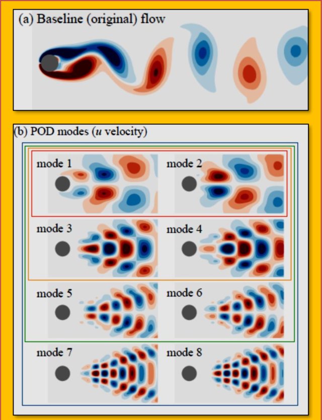
POD refers to the PCA done on the flow data. With a series of snapshots of a flow past a cylinder at \(Re\approx100\), subtracting the mean flow and applying a singular value decomposition (SVA), the resulting dominant eigen flows (modes, representing the flow patterns) can be used to construct a reduced order model to reproduce the fluid flow field efficiently.
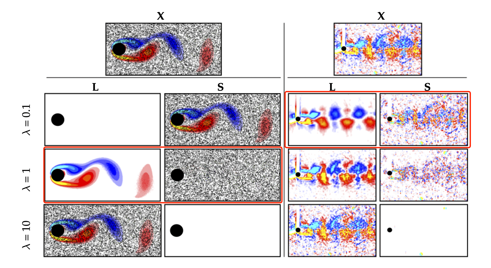
One application of this method is shown below[1], RPCA, a variant of PCA is applied to denoise the artificially pepper-salt corrupted DNS simulation result, and real PIV experiment result. The outliers and the true fluid field are able to separate with a change of the \(\lambda\).
Closure modelling
This is a DNS simulation on turbulent boundary layers by HTL. As we zoom in and out, massive fractal, multi-scale patterns are found in space and time. This happens everytime and everywhere when fluid flowing past a wing, car, or inside an engine. But instead of simulating the full DNS equation i.e. resolving the patterns with all the energy scales, we only want to get a reduced order model approximating the small energy scales while focusing on only the scales of energy that resulting in the macroscopic change of the fluid.
Steve reckons this as the one of the most exciting area where ML can really make a practical impact on everyday industrials. And I heard that after a talk in China, he said a great progress on the area of turbulence might be made in the next 2 decades. (I'm not sure, just heard of it)
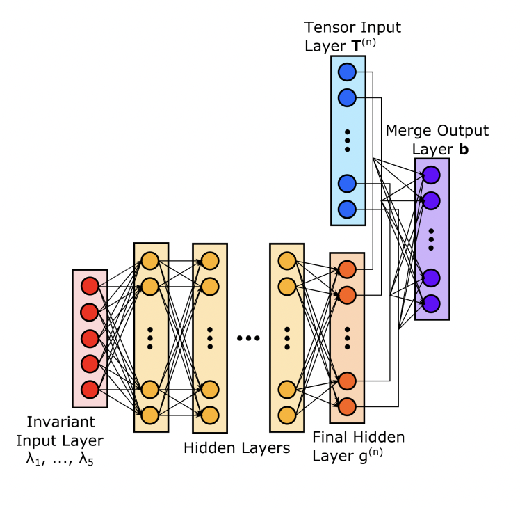
One inspiring job[2] is mentioned which study the RANs closure models. They designed a novel customised structure that embed the physical variables one layer before the output layer of NN. And it inspires us how to "bake in" prior knowledge to design a model not only accurate but also physically meaningful".
Super resolution
Super resolution is already a mature field in image sciences, and it can be directly deployed into flow fields.
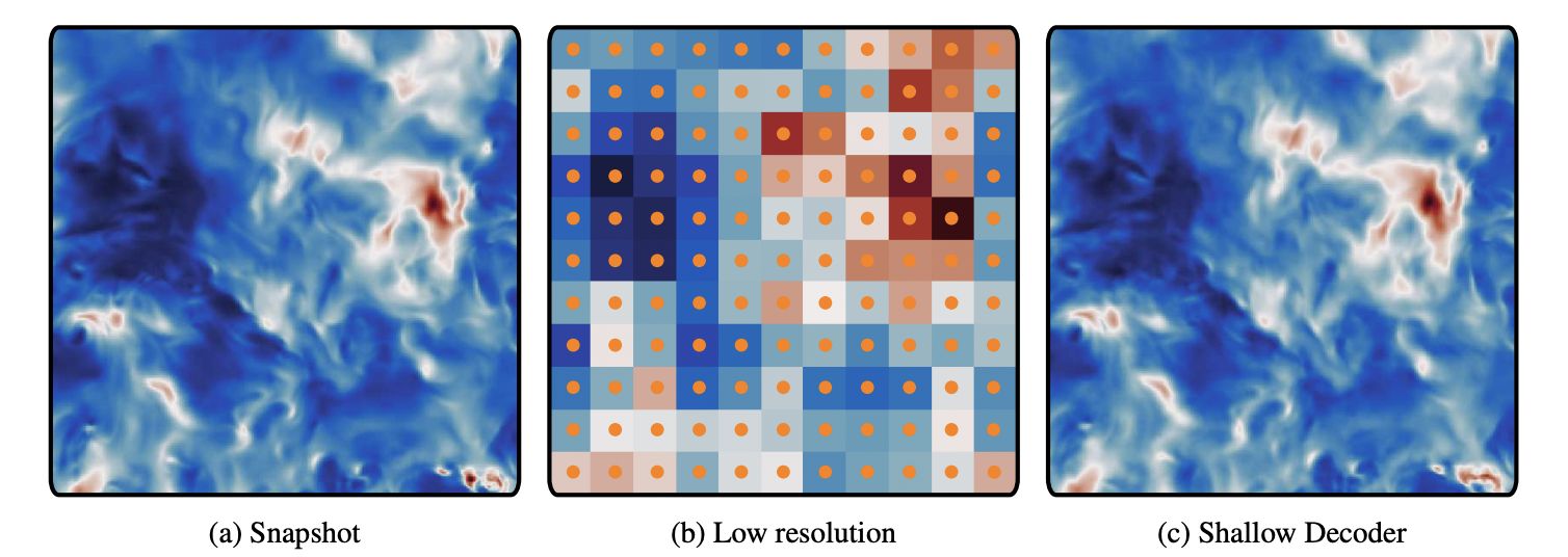
Above is the result of reconstructing the turbulence flow fields(Johns Hopkins Turbulence Database) from the coarse results obtained by applying an average pooling on the original flow fields[3]. Multiple MLPs are deployed for this task.
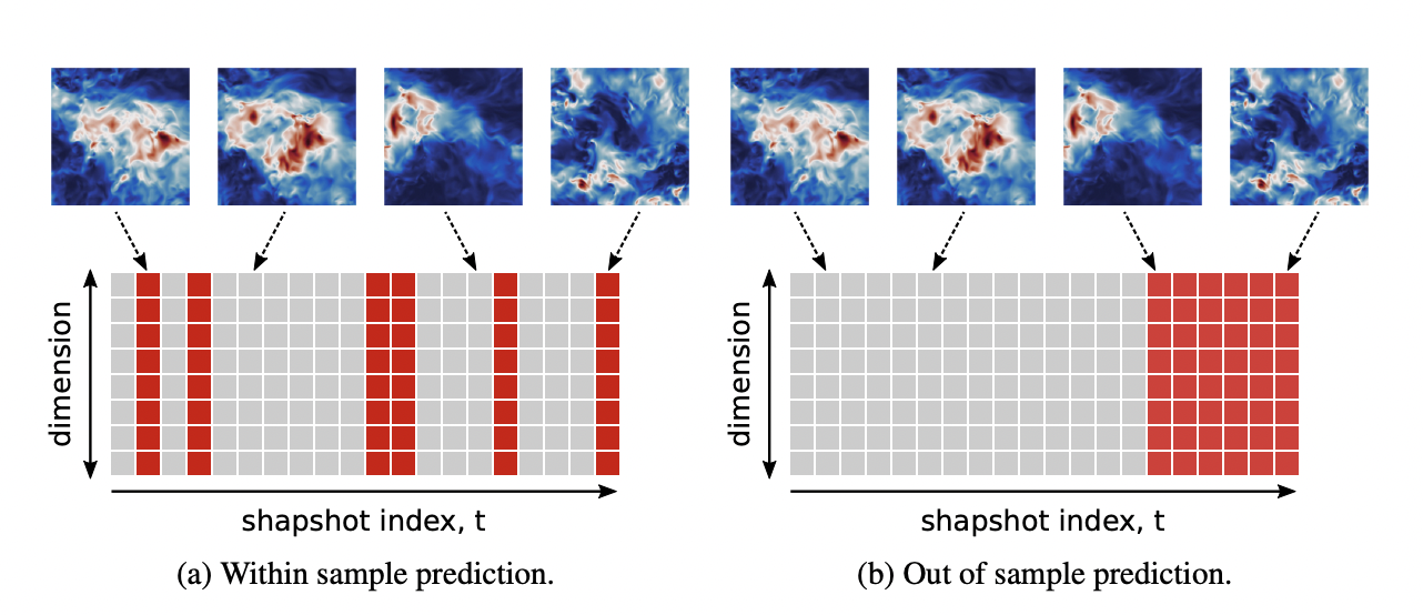
Yet the good results only happen at the interpolation scenario, for the extrapolation i.e. prediction task, the reconstruction failed. More physics need to add to make this work.
Deep autoencoders
The classical POD/PCA can be written in a form of one-layer linear autoencoder. And instead solving by the analytic SVD algorithm, it can be solved by SGD. So why not change the two-layer, linear autoencoder into the non-linear, multilayer deep autoencoder?
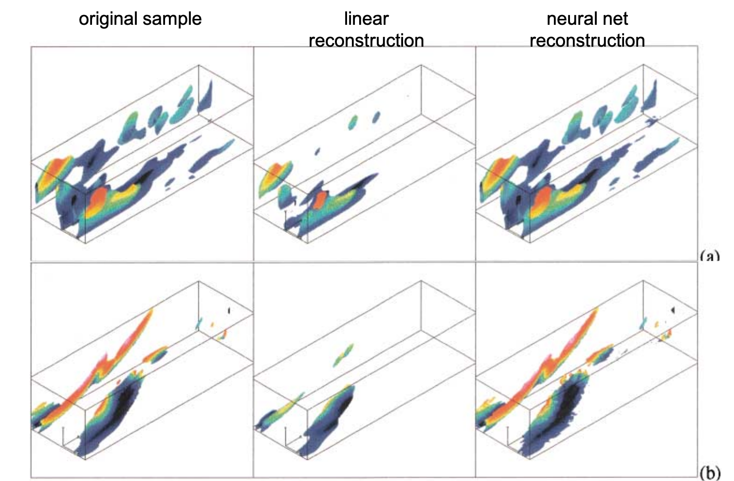
Based on this thought, Michele Milano and Petros Koumoutsakos deployed neural network modeling for near wall turbulent flow[4], and compared with POD results, 2 decades ahead of its time.
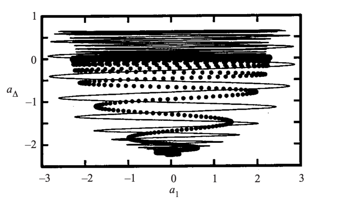
This concepts are also developed to build the reduced order models. The pattens extracted from POD or AE can be used to build simple representations in a low dimensional coordinate. For example Bernd R. Noack et als' work[5] showed the dynamics of transient cylinder wakes can be concluded by a hierarchy of low-dimensional models lived on parabolic bowls.
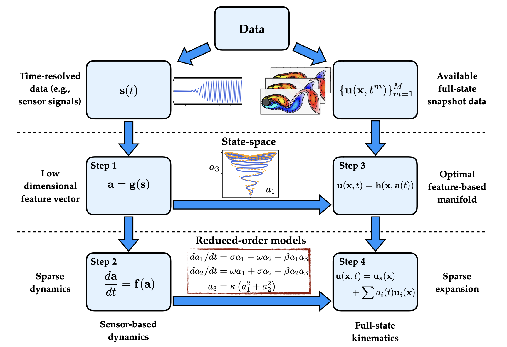
And these learned coordinates can be used with data-diven methods like SINDy(the sparse identification of nonlinear dynamics)[6] to build efficient models for predicting the modes purely from measurement data. Jean-Christophe Loiseau has done a lot work based on this[7].
The ultimate goal: Flow control
It is a very principled optimisation of the flow field and of the control law with some objectives in mind. Those objectives come from the real wold such as: increasing the lift, decreasing the drag. And these optimisation problems can be solved better with machine learning tools.
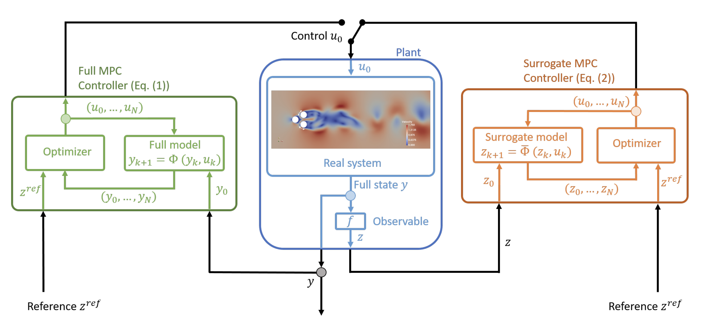
As shown by Bieker at als' diagram[8], instead of controlling a NS equation, an efficient alternative is controlling a machine learning surrogate model to realise the real-time control.
Inspiration from biology
At last to give us some confidence, Steve mentioned without knowing the NS equations, eagle can somehow manoeuvre the complex turbulence flow by its own sensors on its wings. And the insects, with way small neural system, they can handle the complex turbulence flow elegantly and seamlessly (I don't feel any self-confidence hearing this). And maybe we can learn something from them and fit into our engineering world.
- Scherl, I., Strom, B., Shang, J. K., Williams, O., Polagye, B. L., & Brunton, S. L. (2020). Robust principal component analysis for modal decomposition of corrupt fluid flows. Physical Review Fluids, 5(5), 054401. ↩︎
- Ling, J., Kurzawski, A., & Templeton, J. (2016). Reynolds averaged turbulence modelling using deep neural networks with embedded invariance. Journal of Fluid Mechanics, 807, 155-166. ↩︎
- Erichson, N. B., Mathelin, L., Yao, Z., Brunton, S. L., Mahoney, M. W., & Kutz, J. N. (2020). Shallow neural networks for fluid flow reconstruction with limited sensors. Proceedings of the Royal Society A, 476(2238), 20200097. ↩︎
- Milano, M., & Koumoutsakos, P. (2002). Neural network modeling for near wall turbulent flow. Journal of Computational Physics, 182(1), 1-26. ↩︎
- Noack, B. R., Afanasiev, K., MORZYŃSKI, M., Tadmor, G., & Thiele, F. (2003). A hierarchy of low-dimensional models for the transient and post-transient cylinder wake. Journal of Fluid Mechanics, 497, 335-363. ↩︎
- Brunton, S. L., Proctor, J. L., & Kutz, J. N. (2016). Discovering governing equations from data by sparse identification of nonlinear dynamical systems. Proceedings of the national academy of sciences, 113(15), 3932-3937. ↩︎
- Loiseau, J. C., Noack, B. R., & Brunton, S. L. (2018). Sparse reduced-order modelling: sensor-based dynamics to full-state estimation. Journal of Fluid Mechanics, 844, 459-490. ↩︎
- Bieker, K., Peitz, S., Brunton, S. L., Kutz, J. N., & Dellnitz, M. (2019). Deep model predictive control with online learning for complex physical systems. arXiv preprint arXiv:1905.10094. ↩︎