Derivation of Differential Fluid Equations

Feeling unsafe when deploying CFD algorithms, the best way to alleviate the anxiety is to derive the fundamentals again.

1 Acceleration and Mass Conservation

1.1 Acceleration field of a fluid

1.1.1 Material / substantial / convective derivatives

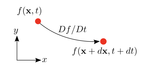
Given a spatial-temporal property \(f(x,y,z,t)\) of a fluid particle in the Eulerian coordinate. After an infinitesimal period, the change in \(f\) , is therefore: \[ \begin{aligned} \Delta f = f(x+\Delta x,y+\delta x,z+\delta z,t+\Delta t)- f(x,y,z,t) \end{aligned} \] set the position and time change tend to 0, \[ \Delta f = \frac{\partial f}{\partial x}\Delta x+\frac{\partial f}{\partial y}\Delta y+\frac{\partial f}{\partial z}\Delta z+\frac{\partial f}{\partial t}\Delta t \] considering: \[ \Delta x = u \Delta t, \Delta y = v \Delta t, \Delta z = w \Delta t \] then \[ \frac{\Delta f }{\Delta t}=\frac{\partial f}{\partial t} + \frac{\partial f}{\partial x}u+\frac{\partial f}{\partial y}v+\frac{\partial f}{\partial z}w \] In the limit as \(\Delta t \rightarrow 0\), \[ \frac{D f }{D t}=\frac{\partial f}{\partial t} + \frac{\partial f}{\partial x}u+\frac{\partial f}{\partial y}v+\frac{\partial f}{\partial z}w \] or in a vector form: \[ \color{purple} \frac{D f }{D t}=\frac{\partial f}{\partial t} + \mathbf{V} \cdot \boldsymbol{\nabla} f \] In the scalar case \(\boldsymbol{\nabla} f\) is simply the gradient of a scalar, while in the vector case, \(\boldsymbol{\nabla} \mathbf{f}\) is the covariant derivative of the vector.

Like the Reynolds Transport Theorem in the integral part, the material derivative connects the Lagrangian and Eulerian frame of references.

1.1.2 Material derivative of velocity

Set \(f\) as \(\mathbf{V}\) and the fluid acceleration as \(\mathbf{a}\), substitute to the formula above: \[ \mathbf{a} = \frac{D \mathbf{V} }{D t}=\underbrace{\frac{\partial \mathbf{V}}{\partial t}}_{\text {local}} + \underbrace{\mathbf{V} \cdot \boldsymbol{\nabla} \mathbf{V}}_{\text {convective}} \] where \(\frac{\partial \mathbf{V}}{\partial t}\) is called local acceleration while \((\mathbf{V} \cdot \boldsymbol{\nabla}) \mathbf{V}\) is the convective acceleration.

It is also written as \(\mathbf{a} = \frac{D \mathbf{V} }{D t}=\frac{\partial \mathbf{V}}{\partial t} + (\mathbf{V} \cdot \boldsymbol{\nabla}) \mathbf{V}\), but it's equivalent.

1.2 Differential equation of mass conservation

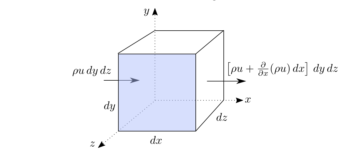
Take an infinitesimally small cubic control volume as below.

With the integral form with one-dimensional assumption: \[ \int_{C V} \frac{\partial \rho}{\partial t} d \mathcal{V}+\sum_{i}\left(\rho_{i} A_{i} V_{i}\right)_{o u t}-\sum_{i}\left(\rho_{i} A_{i} V_{i}\right)_{i n}=0 \]

1. Density can be considered uniform in the CV, \[ \int_{C V} \frac{\partial \rho}{\partial t} d \mathcal{V} = \frac{\partial \rho}{\partial t} dxdydz \]

2. Inlet mass flow in 3 directions \[ \dot{m}_{x} = \rho udydz, \dot{m}_{y} = \rho vdxdz, \dot{m}_{z} = \rho udxdy \]

3. Outlet mass flow in x direction particular \[ \dot{m}_{x+dx} = \left(\rho u+\frac{\partial \rho u}{\partial x }dx\right)dydz \]

4. Substitute all in the continuous function \[ \frac{\partial \rho}{\partial t} dxdydz +\frac{\partial \rho u}{\partial x}dxdydz +\frac{\partial \rho v}{\partial y}dxdydz +\frac{\partial \rho w}{\partial z}dxdydz = 0 \] simplify: \[ \frac{\partial \rho}{\partial t} +\frac{\partial \rho u}{\partial x} +\frac{\partial \rho v}{\partial y} +\frac{\partial \rho w}{\partial z} = 0 \] or in the vector form: \[ \color{purple} \frac{\partial \rho}{\partial t}+\boldsymbol{\nabla} \cdot(\rho\mathbf{V})=0 \]

   The only requirements of this equation are the density \(\rho\) and velocity \(\mathbf{V}\) are continuous in time and space. As a result, this equation is always called the equation of continuity.

1.2.1 Simplifications

• steady flow: \(\partial/\partial t = 0\), \[ \boldsymbol{\nabla} \cdot(\rho\mathbf{V})=0 \]

• Incompressible flow: \(\rho = Const\) spacial and temporal:

\[ \boldsymbol{\nabla} \cdot\mathbf{V}=0 \]

It makes the equation linear and much more tractable to solving analytically.

1.3 Cylindrical coordinates

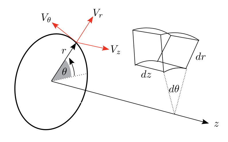
1.3.1 Transformation of coordinates

From cartesian to cylindrical: \[ r=\sqrt{x^{2}+y^{2}} \quad \theta=\tan ^{-1} \frac{y}{x} \quad z=z \]

From cylindrical to cartesian: \[ x=r \cos \theta \quad y=r \sin \theta \quad z=z \]

1.3.2 Differential operators

Two differential operators in polar coordinate: \[ \begin{aligned} \boldsymbol{\nabla} f &=\frac{\partial f}{\partial r} \hat{\boldsymbol{r}}+\frac{1}{r} \frac{\partial f}{\partial \theta} \hat{\boldsymbol{\theta}}+\frac{\partial f}{\partial z} \hat{\boldsymbol{z}}\\ \boldsymbol{\nabla} \cdot \mathbf{V} &=\frac{1}{r} \frac{\partial}{\partial r}\left(r V_{r}\right)+\frac{1}{r} \frac{\partial}{\partial \theta}\left(V_{\theta}\right)+\frac{\partial}{\partial z}\left(V_{z}\right) \end{aligned} \]

6.3.3 Continuous function in cylindrical coordinates

It is easy to substitute the equation of divergence into the continuous function, \[ \frac{\partial \rho}{\partial t}+\frac{1}{r} \frac{\partial}{\partial r}\left(r \rho V_{r}\right)+\frac{1}{r} \frac{\partial}{\partial \theta}\left(\rho V_{\theta}\right)+\frac{\partial}{\partial z}\left(\rho V_{z}\right)=0 \]

2 Linear Momentum and Energy

2.1 Conservation laws from differential Reynolds transport theorem

Recall RTT on a fixed control volume \(\Omega\): \[ \frac{\mathrm{d}}{\mathrm{d} t}\left(B_{s}\right)=\int_{\Omega} \frac{\partial(\beta \rho)}{\partial t} d \mathcal{V}+\int_{\partial \Omega} \beta \rho(\mathbf{V} \cdot \mathbf{n}) d A \] where \[ \beta=\frac{\partial B}{\partial m} \quad \Rightarrow \quad B=\int_{\bar{\Omega}} \beta \rho d \mathcal{V} \] \(\bar{\Omega}\) denotes the control volume in a Lagrangian frame of reference (close system), while \(\Omega\) denotes the control volume in an Eulerian frame of reference (open system).

Open system: matter and energy goes in and out

Close system: energy goes in and out while matter cannot

Isolated system: matter and energy cannot go in and out

In the Lagrangian frame of reference, \[ \frac{\mathrm{d}}{\mathrm{d} t}(B)=\frac{\mathrm{d}}{\mathrm{d} t}\left(\int_{\bar{\Omega}} \beta \rho d \mathcal{V}\right)\underbrace{=}_{Leibniz's Rule}\int_{\bar{\Omega}} \frac{\partial(\beta \rho)}{\partial t} d \mathcal{V}=\int_{\bar{\Omega}} s d \mathcal{V} \]

Leibniz's rule: the derivative moves into the integral symbol: \[\frac{d}{d x}\left(\int_{a}^{b} f(x, t) d t\right)=\int_{a}^{b} \frac{\partial}{\partial x} f(x, t) d t\]

Where \(s\) denotes the "rate of change of \(B\) per unit volume"

Then the RTT is instead: \[ \int_{\bar{\Omega}} s d \mathcal{V} = \int_{\Omega} \frac{\partial(\beta \rho)}{\partial t} d \mathcal{V}+\int_{\partial \Omega} \beta \rho(\mathbf{V} \cdot \mathbf{n}) d A \] Use divergence theorem, drop the bar notation with \(\Delta t \rightarrow 0\), and arrive a differential form: \[ \begin{array}{r} \int_{\Omega} s d \mathcal{V}=\int_{\Omega} \frac{\partial(\beta \rho)}{\partial t} d \mathcal{V}+\int_{\Omega} \boldsymbol{\nabla} \cdot(\beta \rho \mathbf{V}) d \mathcal{V} \\ \int_{\Omega} \frac{\partial(\beta \rho)}{\partial t}+\boldsymbol{\nabla} \cdot(\beta \rho \mathbf{V})-s d \mathcal{V}=0 \\ \Leftrightarrow \color{purple}{\frac{\partial(\beta \rho)}{\partial t}+\boldsymbol{\nabla} \cdot(\beta \rho \mathbf{V})-s=0} \end{array} \]

Divergence theorem: \[\int_{S} \boldsymbol{\nabla} \cdot \mathbf{F} d A=\int_{\partial S} \mathbf{F} \cdot \hat{\mathbf{n}} d s\]

2.1.1 Continuity equation for mass

Substitute \(\beta = 1\) and \(s=0\) (mass created = 0) into the differential RTT: \[ \frac{\partial(\rho)}{\partial t}+\boldsymbol{\nabla} \cdot(\rho \mathbf{V})=0 \] and for incompressible flow: \[ \boldsymbol{\nabla} \cdot \mathbf{V}=0 \]

2.1.2 Continuity equation for linear momentum

Substitute \(\beta =\mathbf{V}\) into the differential RTT: \[ \frac{\partial(\rho \mathbf{V})}{\partial t}+\boldsymbol{\nabla} \cdot(\rho \mathbf{V}\otimes \mathbf{V}) -\mathbf{s} =0 \] \(\mathbf{s}\) denotes the force per unit volume, and $$ denotes the outer product.

Outer product or dyadic product follows: \[\left[\begin{array}{c}u_{1} \\u_{2} \\\vdots \\u_{m}\end{array}\right] \otimes \left[\begin{array}{c}v_{1} \\v_{2} \\\vdots \\v_{n}\end{array}\right]=\left[\begin{array}{cccc}u_{1} v_{1} & u_{1} v_{2} & \ldots & u_{1} v_{n} \\u_{2} v_{1} & u_{2} v_{2} & \ldots & u_{2} v_{n} \\\vdots & \vdots & \ddots & \vdots \\u_{m} v_{1} & u_{m} v_{2} & \ldots & u_{m} v_{n}\end{array}\right]\] The divergence of a dyad follows this formula: \[\begin{aligned}&\boldsymbol{\nabla} \cdot(f \mathbf{a})=(\boldsymbol{\nabla} f) \cdot \mathbf{a}+(\boldsymbol{\nabla} \cdot \mathbf{a}) f \\&\boldsymbol{\nabla} \cdot(\mathbf{a b})=(\boldsymbol{\nabla} \cdot \mathbf{a}) \mathbf{b}+\mathbf{a} \cdot \boldsymbol{\nabla} \mathbf{b}\end{aligned}\]

Expand the equation: \[ \begin{aligned} \rho \frac{\partial \mathbf{V}}{\partial t}+\mathbf{V} \frac{\partial \rho}{\partial t}+\mathbf{V V} \cdot \boldsymbol{\nabla} \rho+\rho \mathbf{V} \cdot \boldsymbol{\nabla} \mathbf{V}+\rho \mathbf{V} \boldsymbol{\nabla} \cdot \mathbf{V} &=\mathbf{s} \\ \Leftrightarrow \mathbf{V}\left(\frac{\partial \rho}{\partial t}+\mathbf{V} \cdot \boldsymbol{\nabla} \rho+\rho(\boldsymbol{\nabla} \cdot \mathbf{V})\right)+\rho\left(\frac{\partial \mathbf{V}}{\partial t}+(\mathbf{V} \cdot \boldsymbol{\nabla} ) \mathbf{V}\right) &=\mathbf{s} \end{aligned} \] With \(\mathbf{V} \cdot \boldsymbol{\nabla} \rho+\rho(\boldsymbol{\nabla} \cdot \mathbf{V})=\boldsymbol{\nabla} \cdot(\rho \mathbf{V})\), we have the first left term a continuity equation. Drop it we have: \[ \mathbf{V}\underbrace{\left(\frac{\partial \rho}{\partial t}+\boldsymbol{\nabla} \cdot(\rho \mathbf{V})\right)}_{0}+ \rho\underbrace{\left(\frac{\partial \mathbf{V}}{\partial t}+(\mathbf{V} \cdot \boldsymbol{\nabla} ) \mathbf{V}\right)}_{\mathrm{material~derivative}} =\mathbf{s} \] With the definition of material derivative, \[ \color{purple} \rho\left(\frac{D \mathbf{V}}{D t}\right) =\mathbf{s} \] Without source or sink, the quantity \(\mathbf{s}\) therefore represents ”force per unit volume“ \(\mathbf{s}=\frac{\mathrm{d} \mathbf{F}}{\mathrm{d} \mathcal{V}}\).

2.2 Forces

The forces contain body forces and surface forces \(\mathbf{F}=\mathbf{F_b}+\mathbf{F_s}\),

• Body forces are due to external fields, take gravitational force as an example, \[ d \mathbf{F}_{g}=\rho \mathbf{g} d x d y d z \quad \mathbf{g}=-g \mathbf{k} \] Consider the only body force in fluid dynamic is the gravity: \[ \color{purple} \frac{\mathrm{d}\mathbf{F_b}}{\mathrm{d}\mathcal{V}} = \rho\mathbf{g} \]

• Surface forces are due to hydrostatic pressure and viscous stresses on the CS: \[ \sigma_{i j}=\left|\begin{array}{ccc} -p+\tau_{x x} & \tau_{y x} & \tau_{z x} \\ \tau_{x y} & -p+\tau_{yy} & \tau_{z y} \\ \tau_{x z} & \tau_{y z} & -p+\tau_{z z} \end{array}\right| \]

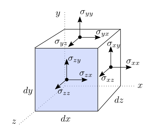
  Similar to what we do in the Mass Conservation, the force is due to the stress change in each direction, for instance: \[ dF{s,xx} = \left(\sigma_{xx}+\frac{\partial\sigma_{xx}}{\partial x}dx\right)dydz-\sigma_{xx}dydz = \frac{\partial\sigma_{xx}}{\partial x}d\mathcal{V} \]

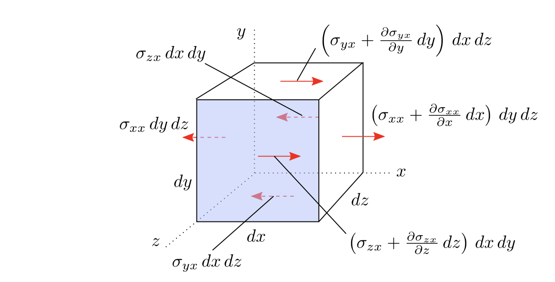
  as a result: \[ \begin{aligned} &\frac{\mathrm{d} F_{x}}{\mathrm{~d} \mathcal{V}}=-\frac{\partial p}{\partial x}+\frac{\partial \tau_{x x}}{\partial x}+\frac{\partial \tau_{y x}}{\partial y}+\frac{\partial \tau_{z x}}{\partial z} \\ &\frac{\mathrm{d} F_{y}}{\mathrm{~d} \mathcal{V}}=-\frac{\partial p}{\partial y}+\frac{\partial \tau_{x y}}{\partial x}+\frac{\partial \tau_{y y}}{\partial y}+\frac{\partial \tau_{z y}}{\partial z} \\ &\frac{\mathrm{d} F_{z}}{\mathrm{~d} \mathcal{V}}=-\frac{\partial p}{\partial z}+\frac{\partial \tau_{x z}}{\partial x}+\frac{\partial \tau_{y z}}{\partial y}+\frac{\partial \tau_{z z}}{\partial z} \end{aligned} \] surface force in vector form: \[ \color{purple} \frac{\mathrm{d} \mathbf{F_s}}{\mathrm{d} \mathcal{V}}=- \boldsymbol{\nabla} p+ \boldsymbol{\nabla} \cdot\boldsymbol{\tau_{ij}} \] \(\frac{\mathrm{d} \mathbf{F_s}}{\mathrm{d} \mathcal{V}}\) also represents the Cauchy stress tensor:

2.3 General differential linear momentum equation

Substitute force terms into earlier momentum conservation expression, \[ \color{purple} \rho\frac{D \mathbf{V}}{D t} = \rho\mathbf{g} - \boldsymbol{\nabla} p+ \boldsymbol{\nabla} \cdot\mathbf{\tau_{ij}} \]

\[ \mathrm{density × acceleration = (Gravity + Pressure + Viscous) ~forces~per~unit~volume} \]

These equations are valid for any fluid in general motion, particularly those which include viscous stresses. The non-linear convective terms on the left-hand side also complicates direct mathematical analysis.

2.4 Differential energy equations

Similar to earlier routes, we arrive energy conservation equation: \[ \dot{Q}-\dot{W}_{v}=\left(\rho \frac{D e}{D t}+\mathbf{V} \cdot \boldsymbol{\nabla} p+p \boldsymbol{\nabla} \cdot \mathbf{V}\right) \mathrm{d}\mathcal{V} \] Note that \(\dot{W}_{s} = 0\) since there is no shaft work in an infinitesimal CV, as a result, similar CV flux analysis can be done to \(\dot{Q}\) and \(\dot{W}_{v}\):

• Heat conduction \(\dot{Q}\) is regulated by Fourier's law stating that the heat flux is proportional to the gradient of the temperature, \(\mathbf{q} = K\boldsymbol{\nabla}T\), using similar flux analysis to infinitesimal CV： \[ \dot{Q}=\boldsymbol{\nabla} \cdot(k \boldsymbol{\nabla} T)\mathrm{d}\mathcal{V} \]

• Similarly, the rate of work due to viscous stresses can be expanded to give: \[ \dot{W}_{v}=-\boldsymbol{\nabla} \cdot\left(\mathbf{V} \cdot \boldsymbol{\tau}_{i j}\right)\mathrm{d}\mathcal{V} \]

Substitute into energy conservation equation to give: \[ \rho \frac{D e}{D t}+\mathbf{V} \cdot \boldsymbol{\nabla} p+p \boldsymbol{\nabla} \cdot \mathbf{V} = \boldsymbol{\nabla} \cdot(k \boldsymbol{\nabla} T) +\boldsymbol{\nabla} \cdot\left(\mathbf{V} \cdot \boldsymbol{\tau}_{i j}\right) \]

2.4.1 General energy equation

Splitting the viscous work term: \[ \boldsymbol{\nabla} \cdot\left(\mathbf{V} \cdot \boldsymbol{\tau}_{i j}\right) \equiv \mathbf{V} \cdot \left( \boldsymbol{\nabla} \cdot \boldsymbol{\tau_{ij}} \right) + \underbrace{\boldsymbol{\tau_{ij}} : \left( \boldsymbol{\nabla}\mathbf{V} \right)}_{\boldsymbol{\Phi}} \] where \(\boldsymbol{\Phi}\) denotes the viscous-dissipation function, representing the dissipation of energy due to viscous effects. For Newtonian flow in a Cartesian coordinates: \[ \boldsymbol{\Phi}=\mu\left[2\left(\frac{\partial u}{\partial x}\right)^{2}+2\left(\frac{\partial v}{\partial y}\right)^{2}+2\left(\frac{\partial w}{\partial z}\right)^{2}+\left(\frac{\partial v}{\partial x}+\frac{\partial u}{\partial y}\right)^{2}+\left(\frac{\partial w}{\partial y}+\frac{\partial v}{\partial z}\right)^{2}+\left(\frac{\partial u}{\partial z}+\frac{\partial w}{\partial x}\right)^{2}\right] \]

Dissipated energy means during the flow, it is converted into the internal energy of the material. Note \(\boldsymbol{\Phi}\) is always positive, implying that viscous flow always loses energy.

Expanding \(e = \hat{u}+\frac{1}{2}V^{2}+gz\), the general differential energy equation is : \[ \color{purple} \rho \frac{D \hat{u}}{D t}+p(\boldsymbol{\nabla} \cdot \mathbf{V})=\boldsymbol{\nabla} \cdot(k \boldsymbol{\nabla} T)+\mathbf{\Phi} \] with further assumptions: \[ \begin{aligned} d \hat{u} & \approx c_{v} d T \\ c_{v}, \mu, k, \rho & \approx \mathrm{const} \end{aligned} \] for incompressible flow, we have: \[ \color{purple}{\rho c_{v} \frac{\partial T}{\partial t} =\cdot(k \boldsymbol{\nabla}^2 T)+\mathbf{\Phi}} \]

3 Euler and Navier-Stokes Equations

Recall differential linear momentum equation: \[ \rho\mathbf{g} - \boldsymbol{\nabla} p+ \boldsymbol{\nabla} \cdot\boldsymbol{\tau_{ij}} = \rho\frac{D \mathbf{V}}{D t} \] Equations of motion of \(\boldsymbol{\tau_{ij}}\) is still needed, and its different depending on types of fluid

3.1 Euler equations (frictionless flow)

Use the inviscid flow assumption, that is \(\boldsymbol{\tau_{ij}}=0\), the momentum equation reduces to: \[ \color{purple} \rho\mathbf{g} - \boldsymbol{\nabla} p+ \boldsymbol{\nabla} \cdot\boldsymbol{\tau_{ij}} = \rho\frac{D \mathbf{V}}{D t} \]

Fluids with low viscosity can be reasonably modelled as inviscid, except near boundaries.

3.2 Newtonian fluid

3.2.1 Strain

Strains of a fluid particle evaluate the deformation due to an applied shear stress.

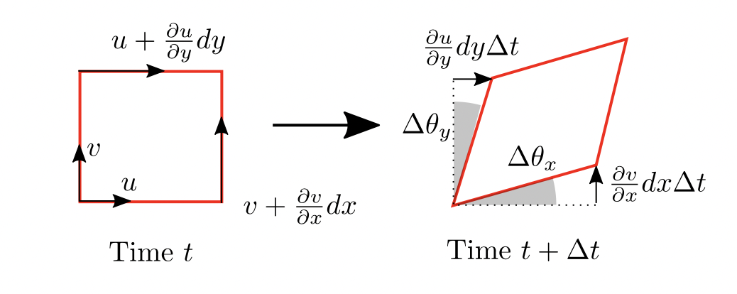
and strain is defined as (anticlockwise positive): \[ \mathrm{strain_{xy}} = \Delta\theta_x-(-\Delta\theta_y) \] In a continuous system, the rate of strain is then: \[ \frac{\mathrm{d}}{\mathrm{d}t}(\mathrm{strain_{xy}}) = \epsilon_{xy} = \frac{\partial v}{\partial x} + \frac{\partial u}{\partial y} \] or in vector form: \[ \boldsymbol{\epsilon} = \nabla \mathbf{V}+(\nabla \mathbf{V}^{\top}) \]

3.2.2 Viscosity

Newton defined a newtonian fluid by a fluid in which the viscous stresses are linearly proportional to the local strain rates. \[ \boldsymbol{\tau_{ij}} \propto \boldsymbol{\epsilon_{ij}} \] In order to apply this to the Naiver–Stokes equations, three assumptions were made by Stokes:

• The stress tensor is a linear function of the strain rate tensor or equivalently the velocity gradient.
• The fluid is isotropic.
• For a fluid at rest, \(\boldsymbol{\nabla} \cdot\boldsymbol{\tau_{ij}} = 0\) (so that hydrostatic pressure results).

And it leads to: \[ \color{purple} \boldsymbol{\tau}=\mu\left(\nabla \mathbf{u}+\nabla \mathbf{u}^{\top}\right)+\lambda(\nabla \cdot \mathbf{u}) \mathbf{I} \] or \[ \boldsymbol{\tau_{ij}}=\mu\left(\frac{\partial u_{i}}{\partial x_{j}}+\frac{\partial u_{j}}{\partial x_{i}}\right)+\delta_{i j} \lambda \frac{\partial u_{k}}{\partial x_{k}} \\ \] where, \[ \delta_{i j}= \begin{cases}0 & \text { if } i \neq j \\ 1 & \text { if } i=j\end{cases} \] As a result, expand the formula: \[ \boldsymbol{\tau_{ij}}=\left|\begin{array}{ccc} 2 \mu \frac{\partial u}{\partial x}+\lambda \frac{\partial u_{}}{\partial x_{k}} & \mu\left(\frac{\partial u}{\partial y}+\frac{\partial v}{\partial x}\right) & \mu\left(\frac{\partial u}{\partial z}+\frac{\partial w}{\partial x}\right) \\ \mu\left(\frac{\partial v}{\partial x}+\frac{\partial u}{\partial y}\right) & 2 \mu \frac{\partial v}{\partial y}+\lambda \frac{\partial v}{\partial y} & \mu\left(\frac{\partial v}{\partial z}+\frac{\partial w}{\partial y}\right) \\ \mu\left(\frac{\partial w}{\partial x}+\frac{\partial u}{\partial z}\right) & \mu\left(\frac{\partial w}{\partial y}+\frac{\partial v}{\partial z}\right) & 2 \mu \frac{\partial w}{\partial z}+\lambda \frac{\partial w}{\partial z} \end{array}\right| \] And \(\mu\) and \(\lambda\) represents the shear/dynamic viscosity and volume/bulk viscosity respectively,

The value of λ, which produces a viscous effect associated with volume change, is very difficult to determine, not even its sign is known with absolute certainty. Even in compressible flows, the term involving λ is often negligible; however it can occasionally be important even in nearly incompressible flows and is a matter of controversy. When taken nonzero, the most common approximation is λ ≈ −2/3μ.

3.3 Navier-Stokes equations

Substitute the stress representation into the linear momentum equation: \[ \rho\frac{D \mathbf{V}}{D t} = \rho\mathbf{g} - \boldsymbol{\nabla} p+ \boldsymbol{\nabla} \cdot \mu\left( \left(\boldsymbol{\nabla} \mathbf{V}+\boldsymbol{\nabla} \mathbf{V}^{\top}\right)-\frac{2}{3}(\nabla \cdot \mathbf{V}) \mathbf{I}\right) \] with further simplification we have: \[ \color{purple} \rho \frac{\mathrm{D} \mathbf{V}}{\mathrm{D} t}=\rho\left(\frac{\partial \mathbf{V}}{\partial t}+\mathbf{V} \cdot \nabla \mathbf{V}\right)=-\nabla p+\mu \nabla^{2} \mathbf{V}+\frac{1}{3} \mu \nabla(\nabla \cdot \mathbf{V})+\rho \mathbf{g} \]

3.3.1 Incompressible Navier-Stokes equations

With incompressible flow we have no bulk viscosity so: \[ \boldsymbol{\tau}=\mu\left(\nabla \mathbf{u}+\nabla \mathbf{u}^{\top}\right) \] And the Incompressible Navier-Stokes equations is therefore: \[ \rho\frac{D \mathbf{V}}{D t} = \rho\mathbf{g} - \boldsymbol{\nabla} p+ \boldsymbol{\nabla} \cdot \mu\left( \boldsymbol{\nabla} \mathbf{V}+\boldsymbol{\nabla} \mathbf{V}^{\top}\right) \] with \(\boldsymbol{\nabla} \cdot \mathbf{V}=0\) for incompressible flow: \[ \boldsymbol{\nabla} \cdot \mu\left( \boldsymbol{\nabla} \mathbf{V}+\boldsymbol{\nabla} \mathbf{V}^{\top}\right) = \mu\boldsymbol{\nabla}^2\mathbf{V} \] as a result: \[ \color{purple} \frac{\partial\mathbf{V}}{\partial t} + \mathbf{V} \cdot \nabla \mathbf{V}= \mathbf{g} - \boldsymbol{\nabla}\frac{p}{\rho} + \nu\boldsymbol{\nabla}^2\mathbf{V} \] where \(\nu = \frac{\mu}{\rho}\), called kinetic viscosity

Meaning of each term: \[\overbrace{\underbrace{\frac{\partial \mathbf{V}}{\partial t}}_{\text {Variation }}+\underbrace{(\mathbf{V} \cdot \nabla) \mathbf{V}}_{\text {Convection }}}^{\text {Inertia (per volume) }}= \overbrace{\underbrace{\nu \nabla^{2} \mathbf{V}}_{\text {Diffusion }}\underbrace{-\nabla w}_{\begin{array}{c}\text { Internal } \\\text { source }\end{array}}}^{\text {Divergence of stress }}+\underbrace{\mathbf{g}}_{\begin{array}{c}\text { External } \\\text { source }\end{array}} .\]

Expanding along every coordinates gives that: \[ \begin{align} \frac{\partial u}{\partial t} + u \frac{\partial u}{\partial x} + v\frac{\partial u}{\partial y} + w \frac{\partial u}{\partial z}&= g_x - \frac{1}{\rho}\frac{\partial p}{\partial x} + \nu\left(\frac{\partial^2u}{\partial^2x}+\frac{\partial^2u}{\partial^2y}+\frac{\partial^2u}{\partial^2z}\right) \\ \frac{\partial v}{\partial t} + u \frac{\partial v}{\partial x} + v\frac{\partial v}{\partial y} + w \frac{\partial v}{\partial z}&= g_y - \frac{1}{\rho}\frac{\partial p}{\partial y} + \nu\left(\frac{\partial^2v}{\partial^2x}+\frac{\partial^2v}{\partial^2y}+\frac{\partial^2v}{\partial^2z}\right) \\ \frac{\partial w}{\partial t} + u \frac{\partial w}{\partial x} + v\frac{\partial w}{\partial y} + w \frac{\partial w}{\partial z}&= g_z - \frac{1}{\rho}\frac{\partial p}{\partial z} + \nu\left(\frac{\partial^2w}{\partial^2x}+\frac{\partial^2w}{\partial^2y}+\frac{\partial^2w}{\partial^2z}\right) \end{align} \]

3.3.2 Cylindrical coordinates

Recall the coordinates transformation: \[ r=\sqrt{x^{2}+y^{2}} \quad \theta=\tan ^{-1} \frac{y}{x} \quad z=z \] and the differential operators: \[ \begin{aligned} \boldsymbol{\nabla} f &=\frac{\partial f}{\partial r} \hat{\boldsymbol{r}}+\frac{1}{r} \frac{\partial f}{\partial \theta} \hat{\boldsymbol{\theta}}+\frac{\partial f}{\partial z} \hat{\boldsymbol{z}}\\ \boldsymbol{\nabla} \cdot \mathbf{V} &=\frac{1}{r} \frac{\partial}{\partial r}\left(r V_{r}\right)+\frac{1}{r} \frac{\partial}{\partial \theta}\left(V_{\theta}\right)+\frac{\partial}{\partial z}\left(V_{z}\right)\\ \boldsymbol{\nabla}^2f &= \left(\frac{1}{r} \frac{\partial}{\partial r}\left(r \frac{\partial f}{\partial r}\right)+\frac{1}{r^{2}} \frac{\partial^{2} f}{\partial \theta^{2}}+\frac{\partial^{2} f}{\partial z^{2}}\right) \end{aligned} \] And in z direction \[ \begin{align} \frac{\partial V_r}{\partial t} + V_r \frac{\partial V_r}{\partial r} + V_\theta\frac{1}{r}\frac{\partial V_r}{\partial \theta} + V_z \frac{\partial V_r}{\partial z}&= g_r - \frac{1}{\rho}\frac{\partial p}{\partial r} + \nu\left(\frac{1}{r} \frac{\partial}{\partial r}\left(r \frac{\partial V_{r}}{\partial r}\right)+\frac{1}{r^{2}} \frac{\partial^{2} V_{r}}{\partial \theta^{2}}+\frac{\partial^{2} V_{r}}{\partial z^{2}}\right) \\ \frac{\partial V_\theta}{\partial t} + V_r \frac{\partial V_\theta}{\partial r} + V_\theta\frac{1}{r}\frac{\partial V_\theta}{\partial \theta} + V_z \frac{\partial V_\theta}{\partial z}&= g_\theta - \frac{1}{\rho r}\frac{\partial p}{\partial \theta} + \nu\left(\frac{1}{r} \frac{\partial}{\partial r}\left(r \frac{\partial V_{\theta}}{\partial r}\right)+\frac{1}{r^{2}} \frac{\partial^{2} V_{\theta}}{\partial \theta^{2}}+\frac{\partial^{2} V_{\theta}}{\partial z^{2}}\right) \\ \frac{\partial V_z}{\partial t} + V_r \frac{\partial V_r}{\partial r} + V_\theta\frac{1}{r}\frac{\partial V_z}{\partial \theta} + V_z \frac{\partial V_z}{\partial z}&= g_z - \frac{1}{\rho}\frac{\partial p}{\partial z} + \nu\left(\frac{1}{r} \frac{\partial}{\partial r}\left(r \frac{\partial V_{z}}{\partial r}\right)+\frac{1}{r^{2}} \frac{\partial^{2} V_{z}}{\partial \theta^{2}}+\frac{\partial^{2} V_{z}}{\partial z^{2}}\right) \end{align} \]

3.3 Closing the system

To summarise, the 3 main functions are: \[ \begin{aligned} \frac{\partial \rho}{\partial t}+\nabla \cdot(\rho\mathbf{V}) &=0 & & \text { continuity } \\ \rho \mathbf{g}-\nabla p+\boldsymbol{\nabla} \cdot \boldsymbol{\tau}_{i j} &=\rho \frac{D \mathbf{V}}{D t} & & \text { momentum } \\ \rho \frac{D \hat{u}}{D t}=p(\boldsymbol{\nabla} \cdot \mathbf{V}) &=\boldsymbol{\nabla} \cdot(k \boldsymbol{\nabla} T)+\mathbf{\Phi} & & \text { energy } \end{aligned} \] Note that there are five unknowns \(\rho,\mathbf{V}, p, \hat{u},T\), but only three equations. Additional equations are state relations for the thermodynamic properties of the fluid. For example for perfect gas: \[ \rho=\frac{p}{R T} \quad \hat{u}=\int c_{v} d T \] The system of equations is now well-posed and can be solved, subject to boundary conditions.

3.3.1 Incompressible system

We have: \[ \begin{aligned} \boldsymbol{\nabla} \cdot \mathbf{V} &=0 \\ \rho \frac{D \mathbf{V}}{D t} &=\rho \boldsymbol{g}-\nabla p+\mu \nabla^{2} \mathbf{V} \\ \rho c_{p} \frac{D T}{D t} &=k \nabla^{2} T+\mathbf{\Phi} \end{aligned} \] Note that for incompressible flow, \(\rho,\mu,k\) are constants, only 3 unknowns are left \(p, \mathbf{V}, T\). So the incompressible system is already closed. Besides, continuity and momentum equations are independent of the \(T\), thus decouple from the energy equation.

3.4 Boundary conditions

• Wall: these are typically solid, impermeable and there is a no-slip condition at the wall.
• Inlet: known velocity \(\mathbf{V}\) and pressure \(p\) (and temperature \(T\))

3.5 Stream function

Stream function provides a mathematical tool to automatically satisfy the continuity constraint, after which we can then solve the momentum equation.

It is only applicable to flows which are steady, incompressible and two-dimensional.

With continuity equation: \[ \boldsymbol{\nabla}\cdot\mathbf{V} = 0 \Leftrightarrow \frac{\partial u }{\partial x} + \frac{\partial v}{\partial y} = 0 \] We seek to replace the velocity components \(u\) and \(v\) with a scalar function \(\psi(x,y)\), which satisfies the above constraint: \[ \frac{\partial}{\partial x}\left(\frac{\partial \psi}{\partial y}\right) + \frac{\partial}{\partial y}\left(-\frac{\partial \psi}{\partial x}\right) \equiv 0 \] As a result: \[ u=\frac{\partial \psi}{\partial y} \qquad v=-\frac{\partial \psi}{\partial x} \]

3.5.1 Properties of stream function

• Recall the definition of a streamline:

\[ \begin{align} & \frac{dy}{v} = \frac{dx}{u} \\ \Leftrightarrow\quad & \frac{\partial \psi}{\partial y}u+\frac{\partial \psi}{\partial x}v=0 \\ \Leftrightarrow\quad & d\psi=0 \\ \Leftrightarrow\quad & \psi=Const \end{align} \]

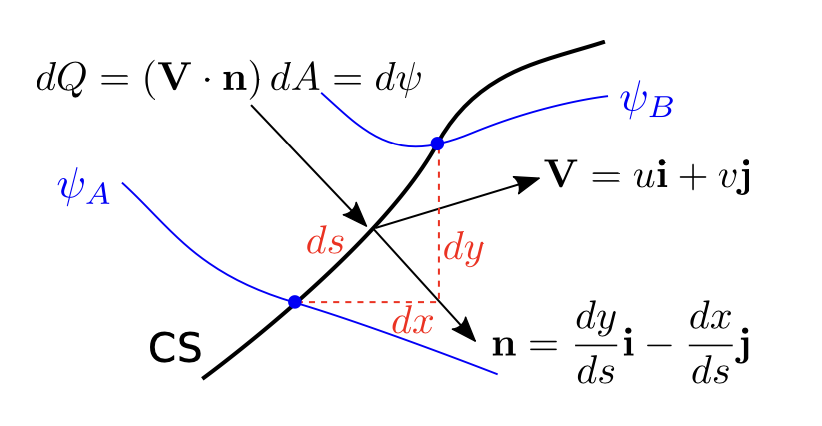
• The change of \(\psi\) across a control surface of unit depth is equal to the volume flow through the surface

  \[ \begin{aligned} d Q &=(\mathbf{V} \cdot \boldsymbol{n}) d A \\ &=\left(\boldsymbol{i} \frac{\partial \psi}{\partial y}-\boldsymbol{j} \frac{\partial \psi}{\partial x}\right) \cdot\left(\boldsymbol{i} \frac{\mathrm{d} y}{\mathrm{~d} s}-\boldsymbol{j} \frac{\mathrm{d} x}{\mathrm{~d} s}\right) d s \\ &=\frac{\partial \psi}{\partial x} d x+\frac{\partial \psi}{\partial y} d y \\ &=d \psi \end{aligned} \]

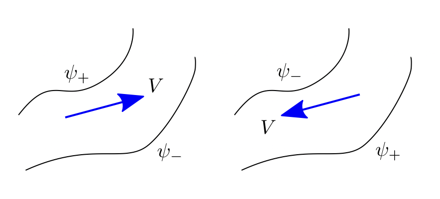
• The flow direction can be determined by observing whether \(\psi\) increases or decreases

  

4 Vorticity and Irrotationality

4.1 Vorticity

Recall how a fluid particle deforms under shear stresses:

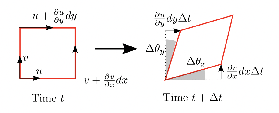
The angular velocity \(\omega_z\) is defined as the average rate of counter-clockwise turning of the two sides: \[ \omega_z = \frac{1}{2}\left(\frac{\mathrm{d}(\Delta\theta_x)}{\mathrm{d}t}+\frac{\mathrm{d}(\Delta\theta_y)}{\mathrm{d}t}\right) =\frac{1}{2}\left(\frac{\partial v}{\partial x}-\frac{\partial u}{\partial y}\right) \] Similarly, \[ \omega_{x}=\frac{1}{2}\left(\frac{\partial w}{\partial y}-\frac{\partial v}{\partial z}\right) \quad \omega_{y}=\frac{1}{2}\left(\frac{\partial u}{\partial z}-\frac{\partial w}{\partial x}\right) \] Combine together the angular velocity: \[ \boldsymbol{\omega}=\frac{1}{2}(\underbrace{\boldsymbol{\nabla} \times \mathbf{V}}_{\text {curl } \mathbf{V}})=\frac{1}{2}\left|\begin{array}{ccc} \mathbf{i} & \mathbf{j} & \mathbf{k} \\ \frac{\partial}{\partial x} & \frac{\partial}{\partial y} & \frac{\partial}{\partial z} \\ u & v & w \end{array}\right| \] And the vorticity is defined as twice the angular velocity i.e. curl of velocity: \[ \boldsymbol{\xi}=2 \boldsymbol{\omega}=\operatorname{curl} \mathbf{V}=\boldsymbol{\nabla} \times \mathbf{V} \]

4.2 Vorticity function for two-dimensional incompressible flow

First some math: \[ \begin{aligned} \boldsymbol{\nabla} \times \boldsymbol{\nabla} \phi & \equiv 0 \qquad\qquad&(4.1) \\ \boldsymbol{\nabla} \times\left(\boldsymbol{\nabla}^{2} \mathbf{V}\right) &=\boldsymbol{\nabla}^{2}(\boldsymbol{\nabla} \times \mathbf{V}) \qquad\qquad&(4.2) \\ (\mathbf{V} \cdot \boldsymbol{\nabla}) \mathbf{V} &=\boldsymbol{\nabla}\left(\frac{1}{2} \mathbf{V} \cdot \mathbf{V}\right)-\mathbf{V} \times \boldsymbol{\xi} \qquad\qquad&(4.3) \\ \boldsymbol{\nabla} \times(\mathbf{V} \times \boldsymbol{\xi}) &=-\boldsymbol{\xi}(\boldsymbol{\nabla} \cdot \mathbf{V})+(\boldsymbol{\xi} \cdot \boldsymbol{\nabla}) \mathbf{V}-(\mathbf{V} \cdot \boldsymbol{\nabla}) \boldsymbol{\xi} \qquad\qquad&(4.4) \end{aligned} \] Recall the incompressible momentum equation: \[ \frac{\partial\mathbf{V}}{\partial t} + \mathbf{V}\cdot\boldsymbol{\nabla}\mathbf{V} = \mathbf{g} -\boldsymbol{\nabla}\left(\frac{p}{\rho}\right) + \nu\boldsymbol{\nabla}^2\mathbf{V} \] Take the curl for each term: \[ \underbrace{\boldsymbol{\nabla} \times\frac{\partial\mathbf{V}}{\partial t} }_{\frac{\partial\boldsymbol{\xi}}{\partial t}}+ \boldsymbol{\nabla} \times \underbrace{\mathbf{V}\cdot\boldsymbol{\nabla}\mathbf{V}}_{\boldsymbol{\nabla}\left(\frac{1}{2} \mathbf{V} \cdot \mathbf{V}\right)-\mathbf{V} \times \boldsymbol{\xi},~\mathrm{by}(4.3)} = \underbrace{\boldsymbol{\nabla} \times\mathbf{g}}_{0} - \underbrace{\boldsymbol{\nabla} \times\boldsymbol{\nabla}\left(\frac{p}{\rho}\right)}_{0,~\mathrm{by} (4.1)}+ \nu\underbrace{\boldsymbol{\nabla} \times\boldsymbol{\nabla}^2\mathbf{V}}_{\boldsymbol{\nabla}^{2}(\boldsymbol{\nabla} \times \mathbf{V}),~ \mathrm{by} (4.2)} \] As a result: \[ \frac{\partial\boldsymbol{\xi}}{\partial t}+ \underbrace{\boldsymbol{\nabla} \times\boldsymbol{\nabla}\left(\frac{1}{2} \mathbf{V} \cdot \mathbf{V}\right)}_{0,~\mathrm{by} (4.1)}-\boldsymbol{\nabla} \times\mathbf{V} \times \boldsymbol{\xi}= \nu\boldsymbol{\nabla}^2\boldsymbol{\xi} \] Apply \((4.4)\) cancel terms due to assumptions: \[ \frac{\partial\boldsymbol{\xi}}{\partial t} +\underbrace{\boldsymbol{\xi}(\boldsymbol{\nabla} \cdot \mathbf{V})}_{0,~\mathrm{steady~incompressible}} -\underbrace{(\boldsymbol{\xi} \cdot \boldsymbol{\nabla}) \mathbf{V}}_{0,~\mathrm{2D~flow}} +(\mathbf{V} \cdot \boldsymbol{\nabla}) \boldsymbol{\xi}= \nu\boldsymbol{\nabla}^2\boldsymbol{\xi} \] Finally, the vorticity function for 2D incompressible flow is: \[ \color{purple} \frac{\partial\boldsymbol{\xi}}{\partial t} +(\mathbf{V} \cdot \boldsymbol{\nabla}) \boldsymbol{\xi}= \frac{D\boldsymbol{\xi}}{D t}= \nu\boldsymbol{\nabla}^2\boldsymbol{\xi} \]

Some of the terms have specific physical interpretations:

• \((\mathbf{V} \cdot \boldsymbol{\nabla}) \boldsymbol{\xi}\) is convection
• \((\boldsymbol{\xi} \cdot \boldsymbol{\nabla}) \mathbf{V}\) is stretching
• \(\nu\boldsymbol{\nabla}^2\boldsymbol{\xi}\) is diffusion

Note that there is no pressure term in the vorticity equation, implying that vorticity dynamics are localised in space.

4.2.1 Combine with continuity equation

Recall the definition of the stream function and take the curl: \[ \begin{aligned} \mathbf{V} &= \mathbf{i}\frac{\partial\psi}{\partial y}-\mathbf{j}\frac{\partial\psi}{\partial x} \\ \boldsymbol{\nabla}\times\mathbf{V} &= -\mathbf{k}\boldsymbol{\nabla}^2\psi = -\mathbf{k}\left( \frac{\partial^2\psi}{\partial x^2} + \frac{\partial^2\psi}{\partial y^2} \right) \end{aligned} \] Substitute these into the vorticity equation, a 4th-order single equation in \(\psi\) arrived: \[ \color{purple} \frac{\partial \psi}{\partial y} \frac{\partial}{\partial x}\left(\nabla^{2} \psi\right)-\frac{\partial \psi}{\partial x} \frac{\partial}{\partial y}\left(\nabla^{2} \psi\right)=\nu \nabla^{2}\left(\nabla^{2} \psi\right) \]

Assumptions made:

• Steady flow
• Incompressible
• Two dimensional

One important special case is when
\[ \boldsymbol{\nabla}^2\psi = \frac{\partial^2\psi}{\partial x^2} + \frac{\partial^2\psi}{\partial y^2} = 0 \] The flow is irrotational.

4.3 Full Bernoulli equations

We now consider a flow which is inviscid (although may still be compressible).

Recall Euler's equation: \[ \frac{\partial\mathbf{V}}{\partial t} + \mathbf{V}\cdot\boldsymbol{\nabla}\mathbf{V} = \mathbf{g} -\frac{1}{\rho}\boldsymbol{\nabla}\left(p\right) \] Expand the convection term by \((4.3)\): \[ \frac{\partial\mathbf{V}}{\partial t} + \boldsymbol{\nabla}\left(\frac{1}{2} V^2\right)+ \underbrace{\boldsymbol{\xi}\times\mathbf{V}}_{\mathbf{a}\times\mathbf{b}=-\mathbf{b}\times\mathbf{a}}- \mathbf{g} +\frac{1}{\rho}\boldsymbol{\nabla}\left(p\right)=0 \] Try to integrate it along an arbitrary trajectory in the flow, dot with a small displacement vector \(d\mathbf{r}\): \[ \left[\frac{\partial\mathbf{V}}{\partial t} + \boldsymbol{\nabla}\left(\frac{1}{2} V^2\right)+ \boldsymbol{\xi}\times\mathbf{V}- \mathbf{g} +\frac{1}{\rho}\boldsymbol{\nabla}\left(p\right)\right]d\mathbf{r}=0 \] The 3^rd term equals 0 when:

• Irrotational flow: \(\mathbf{\xi}\equiv0\)

• No flow: \(\mathbf{V}\equiv0\), not possible

• \(d\mathbf{r}\) is parallel to \(\mathbf{V}\), \(\mathbf{V} \times d \boldsymbol{r} \equiv 0\)

  since \((\boldsymbol{\xi} \times \mathbf{V}) \cdot d \boldsymbol{r} \equiv(\mathbf{V} \times d \boldsymbol{r}) \cdot \boldsymbol{\xi}\)

  our path is a streamline

In order to eliminate the 3^rd term while keeping the flow rotational, we integrate the equation along the streamline segment \(ds\), \[ \begin{aligned} \int_1^2\left[\frac{\partial\mathbf{V}}{\partial t} + \boldsymbol{\nabla}\left(\frac{1}{2} V^2\right)- \mathbf{g} +\frac{1}{\rho}\boldsymbol{\nabla}\left(p\right)\right]ds=0 \\ \int_1^2\frac{\partial\mathbf{V}}{\partial t}ds + \left(\frac{1}{2} V_2^2-\frac{1}{2} V_1^2\right) + g(z_2-z_1) +\int_1^2\frac{1}{\rho}\left(dp\right)=0 \end{aligned} \] Rearrange to get the unsteady Bernoulli equation for compressible flow: \[ \color{purple}\int_1^2\frac{\partial\mathbf{V}}{\partial t}ds+\int_1^2\frac{1}{\rho}\left(dp\right)+ \left(\frac{1}{2} V_2^2-\frac{1}{2} V_1^2\right) + g(z_2-z_1)=0 \] Plus the steady and incompressible conditions, the function reduced to the familiar expression: \[ \color{purple} \frac{p}{\rho}+\frac{1}{2}V^2+gz = Const,~\mathrm{~along~a~streamline} \] Plus the irrotational condition, the 3rd term remains 0 regardless the trajectory, the function becomes: \[ \color{purple} \frac{p}{\rho}+\frac{1}{2}V^2+gz = Const,~\mathrm{~everywhere} \]

4.4 Velocity potential

Vector analysis tells us that if the curl of a vector field is zero then that vector field must itself be the gradient of a scalar function. That is,

The function \(\phi\) is called a potential function. \[ \boldsymbol{\nabla} \times \mathbf{V} \equiv 0 \quad \Rightarrow \quad \mathbf{V}=\boldsymbol{\nabla} \phi \]

Velocity potential \(\phi\) is another scalar function, a complementary to the stream function \(\psi\).

It is applicable only in irrotational flow.

Some useful properties:

• In Cartesian coordinate, it reduce the 3 velocity components \(u\), \(v\), \(w\) into a single scalar: \[ u=\frac{\partial \phi}{\partial x} \quad v=\frac{\partial \phi}{\partial y} \quad w=\frac{\partial \phi}{\partial z} \]

• Line of constant \(\phi\) is called potential lines.

  In two-dimensional flow, potential lines are everywhere orthogonal to the streamlines, because: \[ u=\frac{\partial \psi}{\partial y}=\frac{\partial \phi}{\partial x} \quad v=-\frac{\partial \psi}{\partial x}=\frac{\partial \phi}{\partial y} \] The dot-product of their gradients are: \[ \left[\frac{\partial \psi}{\partial x} \mathbf{i}+\frac{\partial \psi}{\partial y} \mathbf{j}\right] \cdot\left[\frac{\partial \phi}{\partial x} \mathbf{i}+\frac{\partial \phi}{\partial y} \mathbf{j}\right]=u(-v)+u v \equiv 0 \]

• If \(\phi\) exists, substitute the definition into the unsteady Bernoulli equation, \[ \frac{\partial \phi}{\partial t}+\int \frac{d p}{\rho}+\frac{1}{2}|\boldsymbol{\nabla} \phi|^{2}+g z=\mathrm{const} \]

  It is an equation between just two scalar quantities, \(\phi\) and \(p\).

5 Vortex Motion and Applications

Vortices are structures within the flow in which fluid is rotating about an axis line (which may be straight or curved). A vortex line is therefore defined as a line which is always in the same direction as the local vorticity vector \(\boldsymbol{\xi}\).

Similar to streamline, vortex lines \((x, y, z) = (x(s), y(s), z(s))\) are obtained by solving: \[ \frac{dx/ds}{d\xi_x}=\frac{dy/ds}{d\xi_y}=\frac{dz/ds}{d\xi_z} \] Similar to steam tube, vertex lines which pass through a closed curve in space form a vortex tube.

5.1 Circulation

Fluid circulation describes the strength of rotation, or strength of fluid swirling, within a closed contour \(C(t)\). Mathematically it is defined as the integral of velocity along the contour curve: \[ \Gamma=\oint_{C(t)} \mathbf{V} d s=\int_{S} \boldsymbol{\xi} \cdot \boldsymbol{n} d S \]

5.1.1 Material elements and its motion

Consider how a infinitesimal displacement \(d\mathbf{s}\) deforms over a small time \(dt\), illustrated in the diagram below.

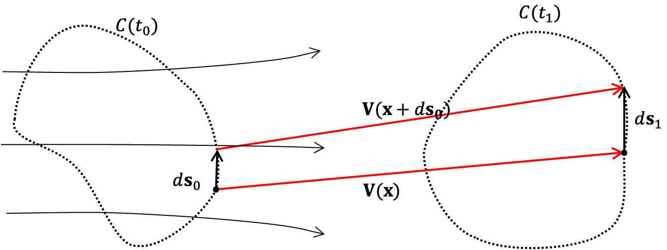
We have \(d(d\mathbf{s})\) the material line element: \[ \begin{aligned} d(d \boldsymbol{s})=d \boldsymbol{s}_{1}-d \boldsymbol{s}_{0} &=\left(\boldsymbol{x}+d \boldsymbol{s}_{0}+\mathbf{V}\left(\boldsymbol{x}+d \boldsymbol{s}_{0}\right) d t\right)-(\boldsymbol{x}+\mathbf{V}(\boldsymbol{x}) d t)-d \boldsymbol{s}_{0} \\ &=\left(\mathbf{V}\left(\boldsymbol{x}+d \boldsymbol{s}_{0}\right)-\mathbf{V}(\boldsymbol{x})\right) d t \\ &=d \boldsymbol{s}_{0} \frac{\partial \mathbf{V}}{\partial\left(d \boldsymbol{s}_{0}\right)} d t \\ &=d \boldsymbol{s}_{0} \cdot \boldsymbol{\nabla} \mathbf{V} d t \end{aligned} \] Therefore: \[ \frac{D(d\mathbf{s})}{Dt} = (ds\cdot\boldsymbol{\nabla})\mathbf{V} \]

5.2 Kelvin’s Circulation Theorem

Kelvin’s Circulation Theorem status the expression of the rate of change of the circulation \(\frac{D\Gamma}{Dt}\) and determine how a circulation around a fluid loop varies as the loop moves with the flow. (reference)

Apply material derivative to circulation we have: \[ \begin{aligned} \frac{D}{Dt}\Gamma&=\frac{D}{Dt}\oint_{C(t)} \mathbf{V} d \mathbf{s} \\ &= \oint_{C(t)}\frac{D}{Dt}(\mathbf{V} d \mathbf{s} ) \\ &= \oint_{C(t)}\frac{D\mathbf{V}}{Dt}\cdot d \mathbf{s} + \oint_{C(t)}\mathbf{V}\cdot \frac{D(d \mathbf{s})}{Dt} \\ \end{aligned} \] Substitute material line element into the last term to get a scalar inside the loop integration, then we have: \[ \frac{D}{Dt}\Gamma = \oint_{C(t)}\frac{D\mathbf{V}}{Dt}d \mathbf{s} \] Recall the general linear momentum equation and substitute the material derivative of velocity: \[ \begin{aligned} \frac{D}{Dt}\Gamma &= \oint_{C(t)}\left(\mathbf{g} - \frac{\boldsymbol{\nabla}p}{\rho} + \frac{\boldsymbol{\boldsymbol{\nabla}\cdot\tau_{ij}}}{\rho}\right)d \mathbf{s} \\ &= \oint_{C(t)}\mathbf{g}d \mathbf{s} - \oint_{C(t)}\frac{\boldsymbol{\nabla}p}{\rho} d\mathbf{s} + \oint_{C(t)}\frac{\boldsymbol{\nabla}\cdot\boldsymbol{\tau_{ij}}}{\rho}d \mathbf{s} \end{aligned} \] This function is not zero unless:

• 1^st term: body force torque is zero, body force is irrotational, \(\mathbf{g} = \nabla\phi\), \(\phi\) is a scalar.
• 2^nd term: \(p = p(\rho)\) or \(\rho = const.\)(incompressible and isotropic)
• 3^rd term: inviscid, \(\boldsymbol{\tau_{ij}}=0\)

5.2.1 Aerofoil lift and Kutta-Joukowski Theorem

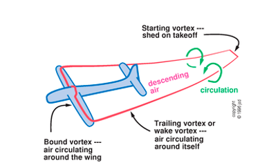
One application of the Kelvin Circulation Theorem is in explaining the lift attained by an aerofoil during the shedding of the starting vortex.

Consider a stationary aerofoil shown in the diagram below.

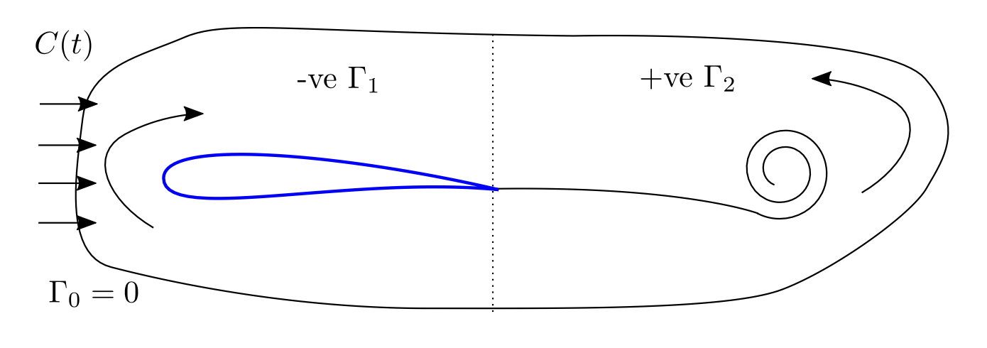
At time \(t = 0\), the aerofoil is stationary, there is no vorticity and around the path \(C(t)\) the circulation is \(\Gamma = 0\). As the flow velocity increases, vorticity is shed behind the aerofoil leading to positive \(\Gamma\).

By Kelvin’s circulation theorem, the circulation \(\Gamma_0\) around \(C(t)\) is independent of time. Therefore, there must be negative \(\Gamma_1\) around the aerofoil, which leads to lift by the Kutta-Joukowski theorem (\(L' = −\rho u\Gamma\)).

5.3 Helmholtz Theorems

Suppose we have an inviscid, incompressible fluid of constant density moving under a conservative body force, then

1. The quantity \[ \Gamma=\int_{S} \boldsymbol{\xi} \cdot \boldsymbol{n} d S \] is the same for all cross-sections \(S\) of a vortex tube. i.e. the strength of a vortex is constant along the length of the vortex.

2. A vortex filament cannot end in the fluid; it must extend to the boundaries of the fluid, infinity, or form a closed loop

3. If fluid is initially irrotational, in the absense of rotational forces, it remains irrotational indefinitely.

5.3.1 Vortex rings

A vivid example of Helmholtz’s theorems can be seen in vortex (smoke) rings. These are vortices in which the core vortex line forms a closed loop (theorem #2).

Such vortices can retain their strength (theorem #1) and travel significant distances (the smoke is carried in the vortex).