Swin transformer
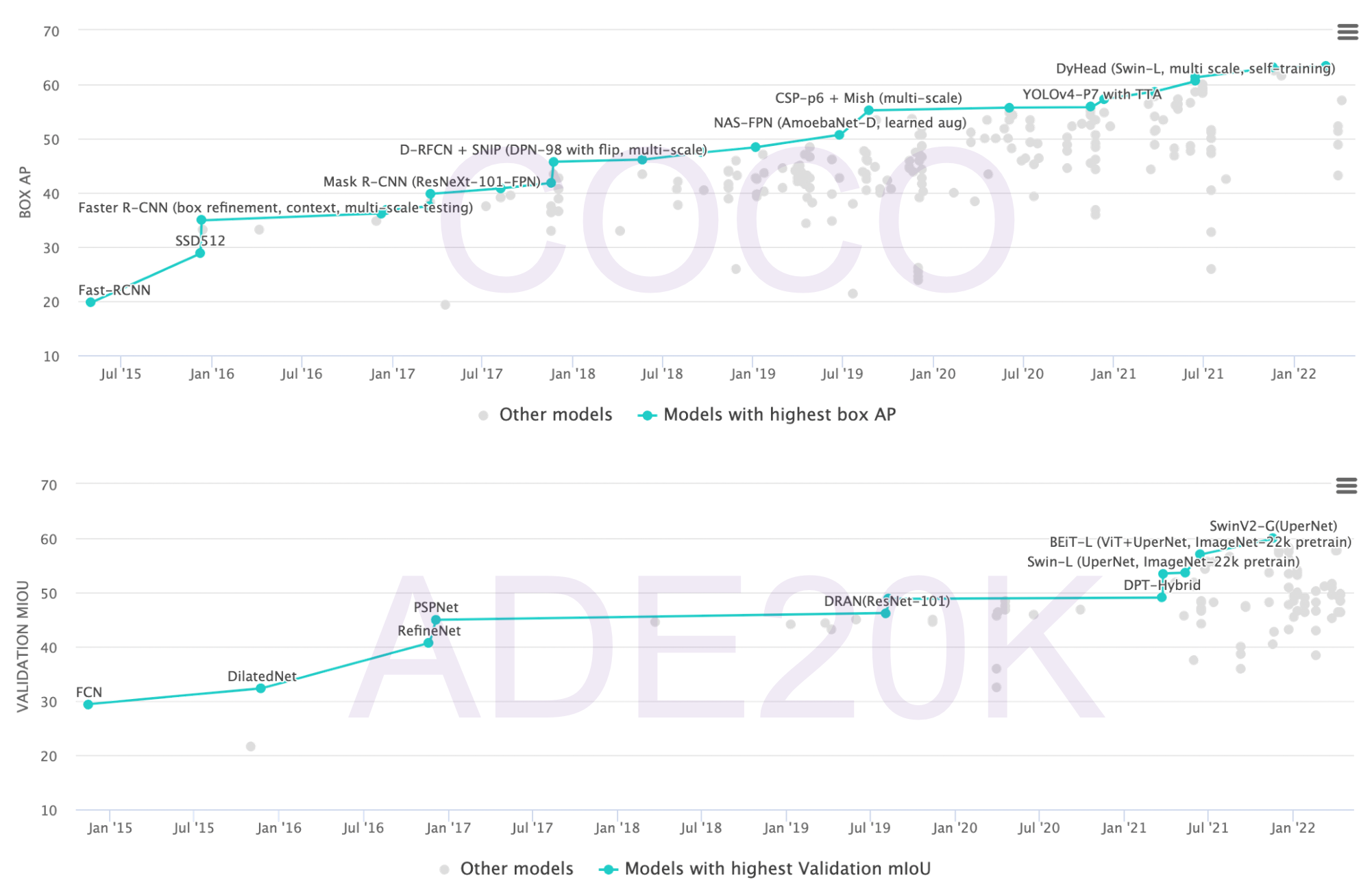
After ViT, Swin-transformer further demonstrated the potential of transformer in CV. This work has swept all major CV tasks since its publication, including COCO and ADE20K. And it's awarded as best paper by ICCV2021.
This is a series of paper reading notes, hopefully, to push me to read paper casually and to leave some record of what I've learned.
Paper link:
Swin Transformer: Hierarchical Vision Transformer using Shifted Windows(newer version on arXiv)
Useful links:
Abstract
It is a general-purpose backbone, unlike ViT which only covers the classification task instead of detection and segmentation. Swin Transformer extends the jobs to all the vision jobs.
Two challenges of using transformer on vision tasks:
- Large scale difference of vision entities (multi-scale)
- high resolution of pixels compared with words (former works use feature map, divide as patch, or self-attention in windows divided from the whole image, to reduce the sequence length)
Main contribution is the Shifted window that brings the Hierarchy to ViT. It has several merits:
- greater efficiency, reduced sequence length
- cross-window connection is allowed with shifted window
- multi-scales
- linear computational complexity with respect to image size, instead of square (foundation for larger Swin Transformer V2, pretrained model on huge resolution)
Many downstream tasks are tested including classification, detection and segmentation.
One line is added to the abstract in this version, after MLPmixer in order to further prove the method of sifted window: shifted window is also beneficial for all-MLP architectures.
Key figures
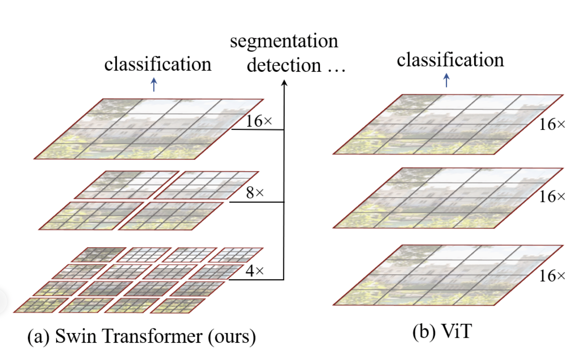
ViT and Swin Transformer are compared in the above illustration, for ViT, the feature map is single and with low resolution (all *16 downsampling \(patchSize = 16\)). For Swin Transformer, the hierarchical feature map is introduced.
Importance of multi-scale feature for detection and segmentation:
For detection, take the most common FPN as an example, features from different layers of feature map of different reception field are collected to ensure the multi scale performance.
For segmentation, take the common UNet as an example, the skip connection of different layers also provide a hierarchy of scales.
Besides, ViT performs self-attention for the whole image, leading to the quadratic computation complexity. Swin transformer instead perform self-attention on the patches. The computational cost for each window is fixed for fixed patch size. As a result the computation complexity is linear.
To some extend, swin transformer takes a lot of prior information of CNNs as:
- the locality inductive bias, i.e. the objects are locally consecutive. The full space self attention is kinda a wast of source.
- For CNN, pooling layers increase the receptive field of each layers, enabling them to catch features with different scales. The patch merging is a mimic of this operation. A bigger patch is merged by 4 smaller patch, so that the receptive field of the bigger patch is increased. The multi scale feature maps can feed a FPN for detection or UNet for segmentation, i.e. a general purpose backbone.
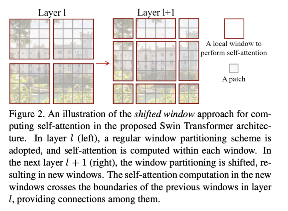
It illustrates how the window is shifted in layers. The unit patch is the grey on with patch size = 4. In the next layer, the window is shifted 2 patches to the right and bottom. The main benefit of this is the ability of cross-window interaction. Without shifting, the self-attention operations are limited to non-overlap patches. The global information is inaccessible, broke the key idea of transformer. The memory can be saved with an ability to global modelling.
1 Introduction
The motivation is to prove the ability of Vision Transformer as a general backbone.
The mechanism is well illustrated from the key figures above.
The good results are next presented.
In future, a unified architecture will benefits both the CV and NLP world. Actually, Swin transformer leverages a lot vision inductive bias to perform well on vision tasks. The unifying is done better for ViT, as it does not change any of the transformer architecture. Very easy for multi modelling learning.
3.Method
3.1 Overall Architecture
Feed forward process and patch merging method are mainly discussed.
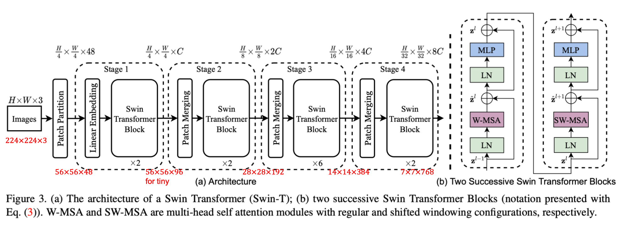
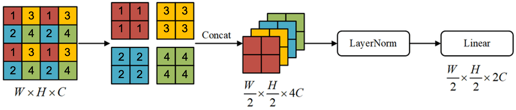
The key process of swin transformer is the patch merging. After merging, the width and height get halved while the length is doubled, just like the convolutional method.
The dimensions of each layer is very similar to CNNs', identical to ResNet. Besides, in order to keep aligned with CNN, the CLS token used in ViT is deprecated.
CLS token is an extra token along with the training tokens in ViT. It contains all the information from every can be directly trained in classification last. For swin transform, the last feature map is flattened into a list, and the result can be used for classification, detection and segmenting, just like CNNs.
There is always a global average pooling layer after the architecture above. For example, if for image classification on ImageNet, the feather length of next two layers are: [1, 768] -> [1, 1000].
3.2 Shifted Window based Self-Attention
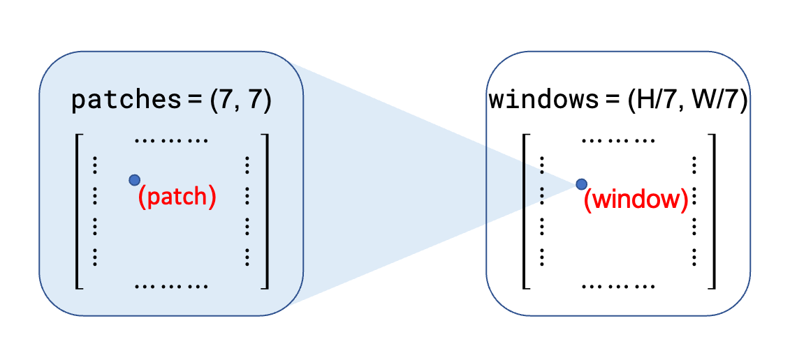
As shown above, the image with \(H \times W\) patches is divided into non-overlapping windows such a way that each window has \(M \times M\) patches (\(M = 7\) for default). The self-attention is computed within each windows, instead of the whole image as in the standard one.
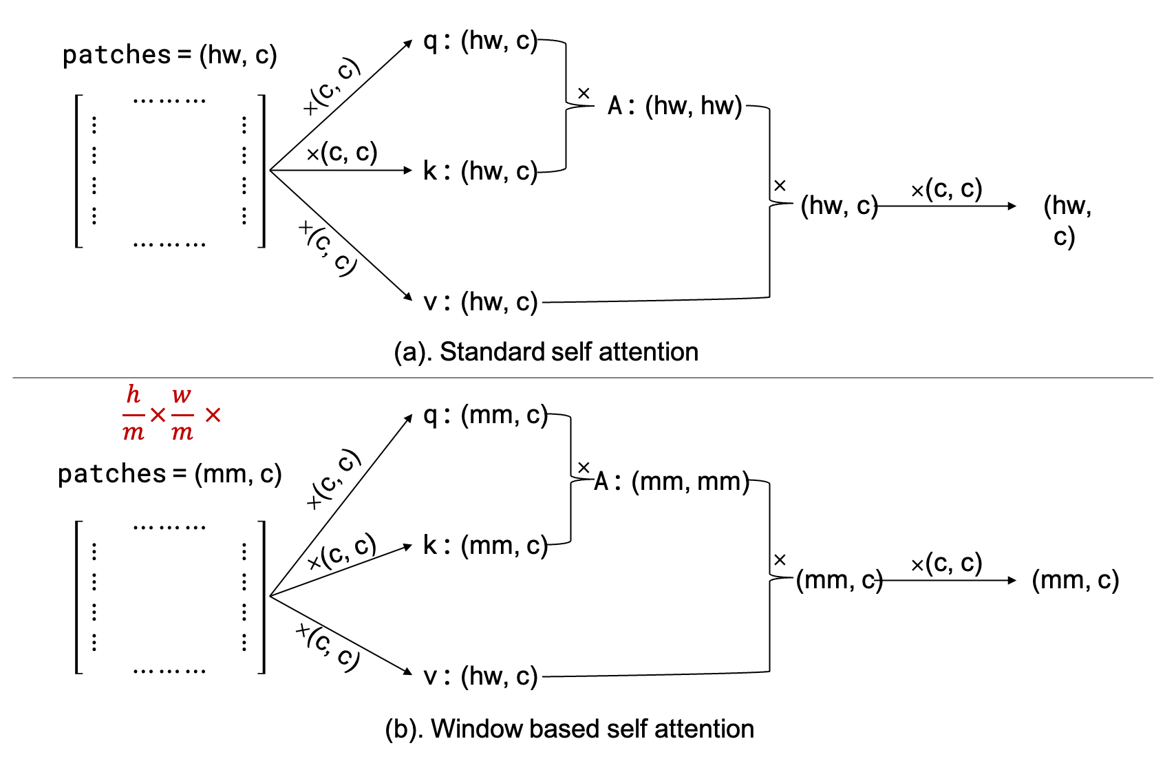
The complexity difference between standard shelf attention (\(\mathrm{MSA}\)) and window base self-attention (\(\mathrm{W}-\mathrm{MSA}\)) is further estimated:
For an image with \(h\times w\) patches: \[ \begin{aligned} &\Omega(\mathrm{MSA})=4 h w C^2+2(h w)^2 C \\ &\Omega(\mathrm{W}-\mathrm{MSA})=4 h w C^2+2 M^2 h w C \end{aligned} \] Note that \(M = 7\), the complexity decrease is huge.
The complexity of the multiplication of two matrices with dimensions \(a\times b\) and \(b \times c\) is \(a\times b \times c\).
After reducing the complexity, the shifting method is introduced to address the problem of cross-window communication, as shown in the key figures and overall architecture sections, a shifted window layer (\(\mathrm{SW}-\mathrm{MSA}\)) always follows a window layer (\(\mathrm{W}-\mathrm{MSA}\)). \[ \begin{aligned} &\hat{\mathbf{z}}^l=\mathbf{W}-\mathbf{M S A}\left(\mathbf{L N}\left(\mathbf{z}^{l-1}\right)\right)+\mathbf{z}^{l-1} \\ &\mathbf{z}^l=\mathbf{M L P}\left(\mathbf{L N}\left(\hat{\mathbf{z}}^l\right)\right)+\hat{\mathbf{z}}^l \\ &\hat{\mathbf{z}}^{l+1}=\mathbf{S W}-\mathbf{M S A}\left(\mathbf{L N}\left(\mathbf{z}^l\right)\right)+\mathbf{z}^l \\ &\mathbf{z}^{l+1}=\mathbf{M L P}\left(\mathbf{L N}\left(\hat{\mathbf{z}}^{l+1}\right)\right)+\hat{\mathbf{z}}^{l+1} \end{aligned} \]
Below is some technical details with shifted window, not related to the main idea of swin-transformer.
Recalling the illustration of shifted windows in key figures, the unlike the window layer, the shifted window layer has more resulting windows (9 instead of 4) with different scales ($2, 4, 4 $), it is impossible to compute efficiently in parallel. Another simple idea is padding, extra 0 is padded so that the scales of windows are identical. But the authors come up with a better one:
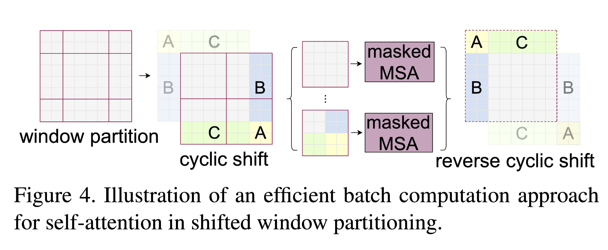
The idea is cyclic shift, pretty much like the periodic boundary condition, the windows out of the "boundary" is glutted back from the left bottom of the image, and after the SW-MSA, a reversed operation is applied. However, unlike the real periodic boundary condition, the glutted windows are actually far from each other, no attention operations should be applied across these windows. In order to do this, the familiar masking technique is introduced
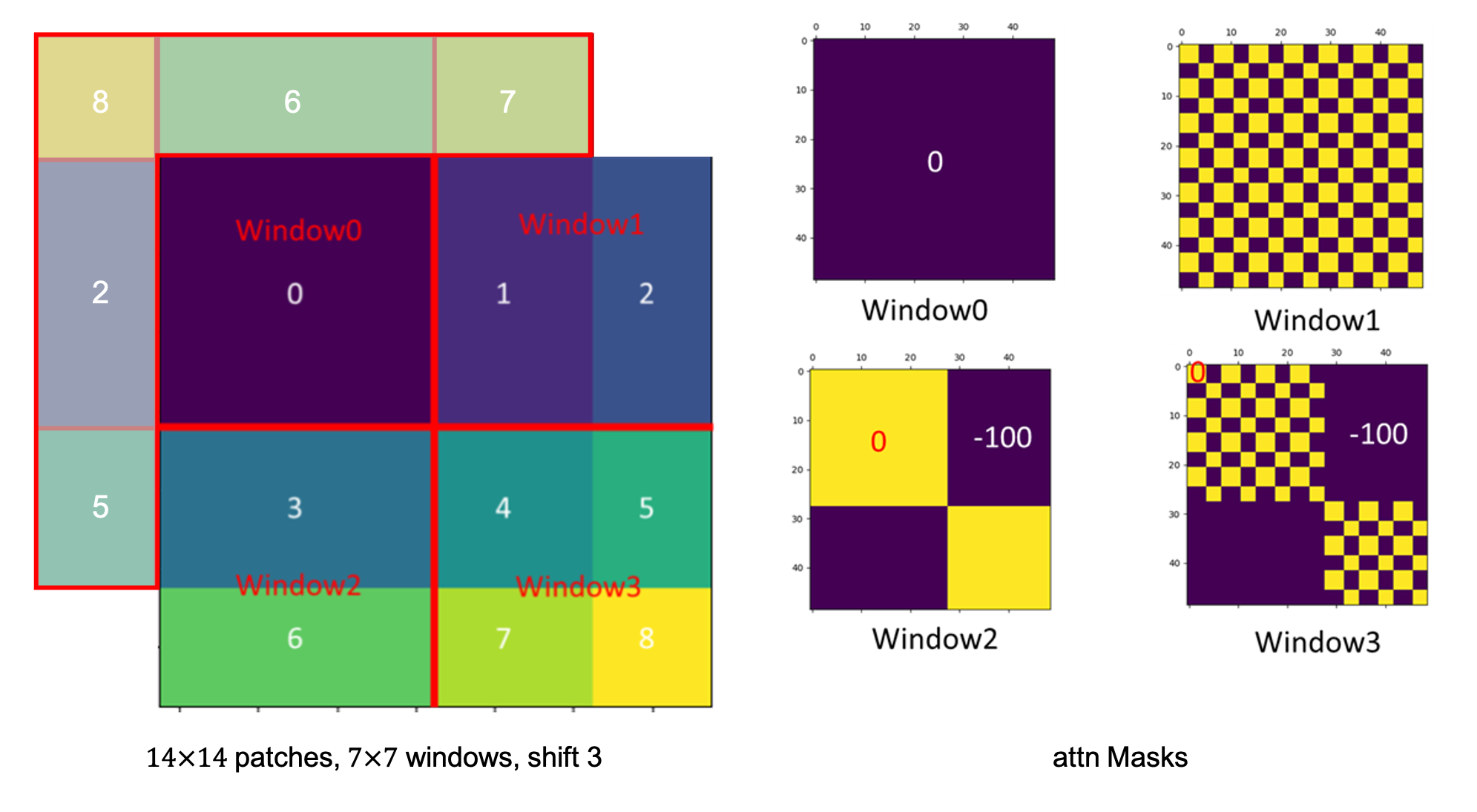
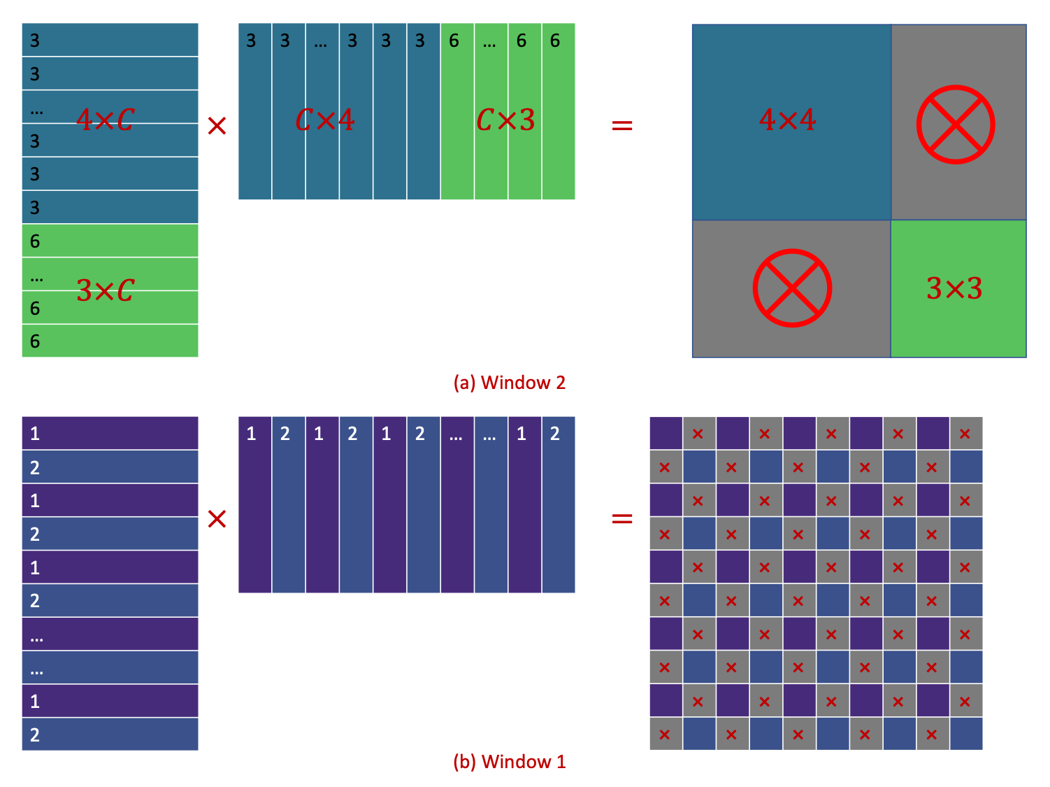
As shown above, for window 2 and 1, only half of the resultant window is useful, the other half needed to be masked. And it is applied by add a mask matrix, where the useful and masked area are set to be \(0\) and \(-100\), respectively. After softmax, the infinite negative number results in 0.
3.3 Architecture variants
Different \(C\) and block numbers of 4 stages differs the variants.
- Swin-T: \(C=96\), layer numbers \(=\{2,2,6,2\}\) -- ResNet50
- Swin-S: \(C=96\), layer numbers \(=\{2,2,18,2\}\) -- ResNet101
- Swin-B: \(C=128\), layer numbers \(=\{2,2,18,2\}\)
- Swin-L: \(C=192\), layer numbers \(=\{2,2,18,2\}\)
5 Conclusion
Swin transformer is presented with linear increase of computational complexity. Good results are shown not only on classification, but in dense tasks such as detection and segmentation.
Patch merging is introduced to percept a hierarchical of feature maps as in CNNs, better for resolving features with a range of scales of an image.
A key element is self attention based on window followed by shifted windows, which is very help for dense tasks.
As the extra shifted window mechanism breaks the potential of multi modelling learning. They are working on use this technique to NLP fields.